The “Runs” of Production
“Time”-frame usefully divided between short vs. long run analysis
Short run: at least one factor of production is fixed (too costly to change) q=f(ˉk,l)
- Assume capital is fixed (i.e. number of factories, storefronts, etc)
- Short-run decisions only about using labor

The "Runs" of Production
"Time"-frame usefully divided between short vs. long run analysis
Long run: all factors of production are variable (can be changed) q=f(k,l)
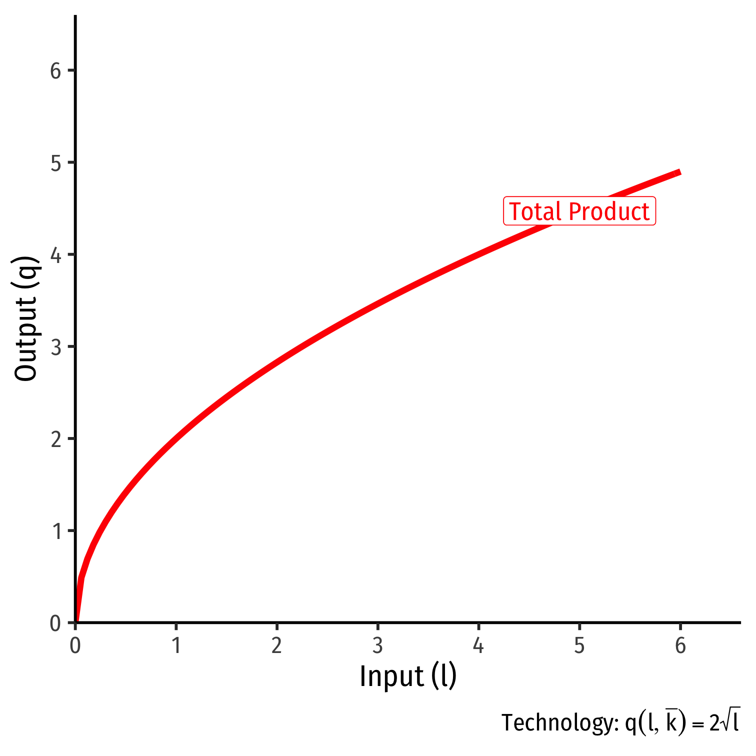
Production in the Short Run: Example
Example: Consider a firm with the production function q=k0.5l0.5
- Suppose in the short run, the firm has 4 units of capital.
- Derive the short run production function.
- What is the total product (output) that can be made with 4 workers?
- What is the total product (output) that can be made with 5 workers?
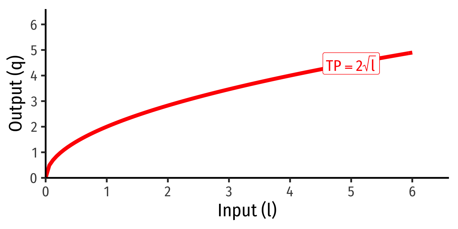
Marginal Products
The marginal product of an input is the additional output produced by one more unit of that input (holding all other inputs constant)
Like marginal utility
Similar to marginal utilities, I will give you the marginal product equations
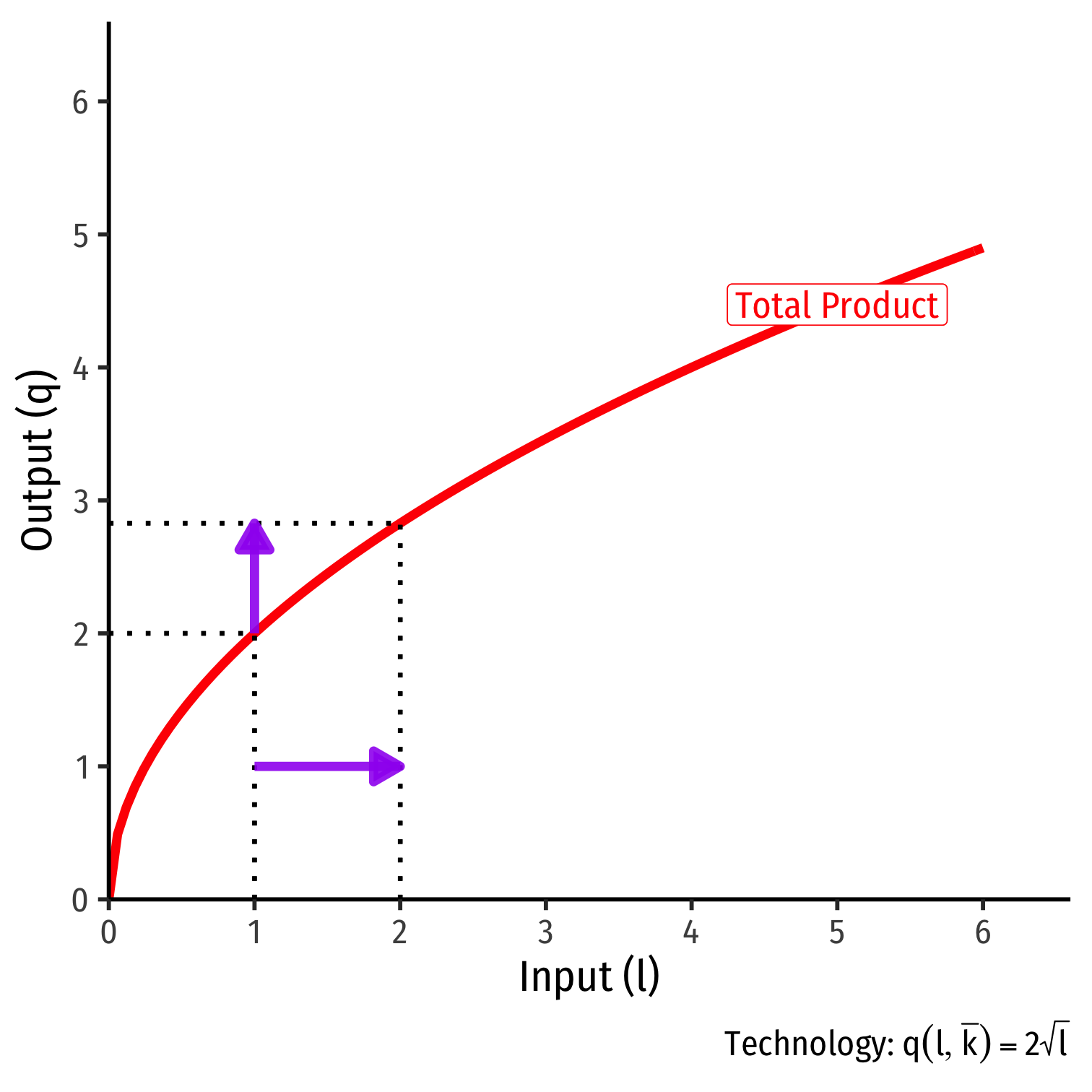
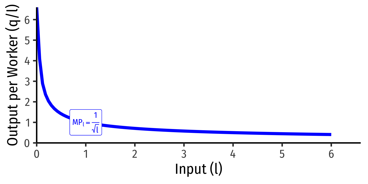
Marginal Product of Labor
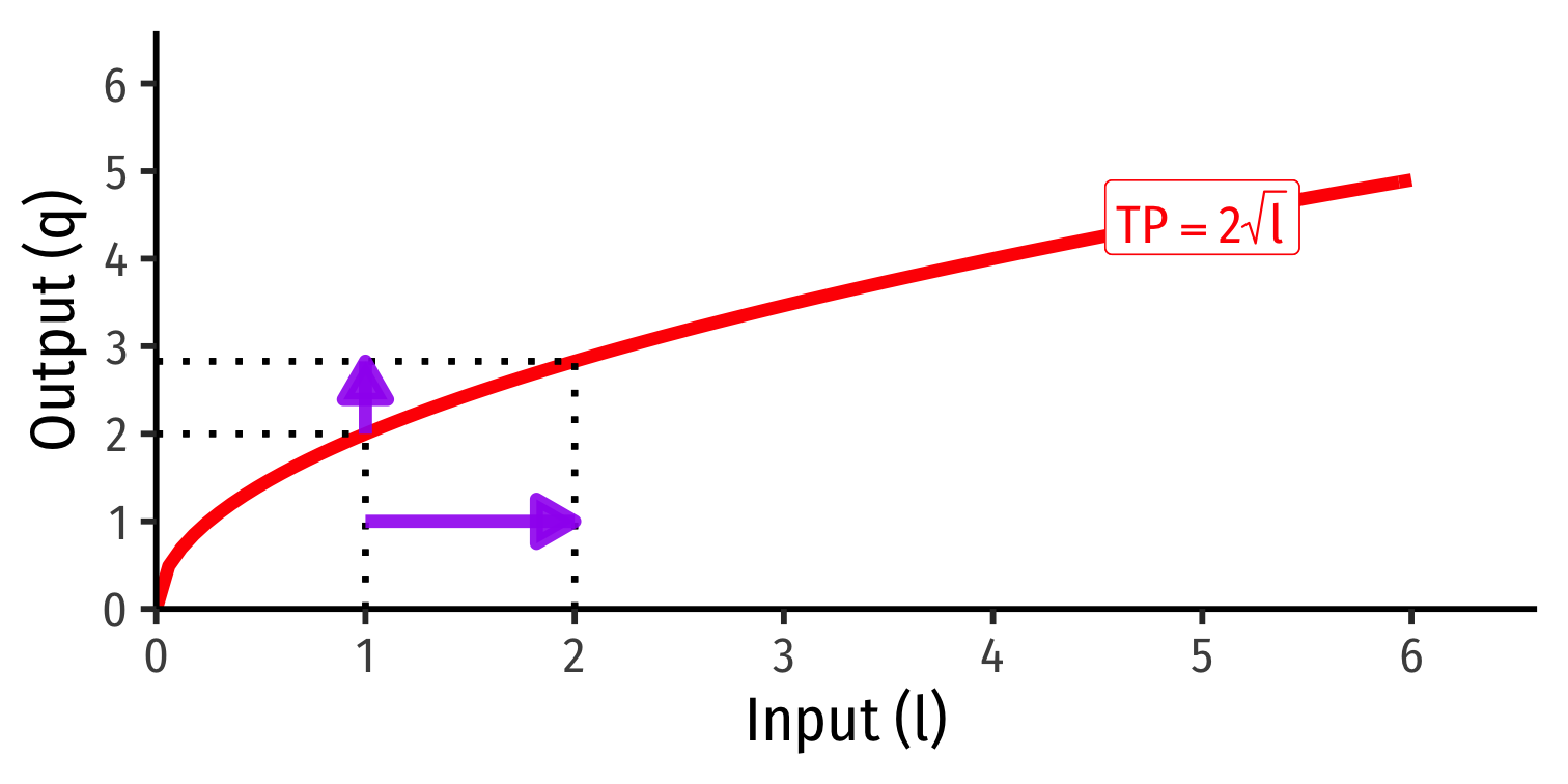
Marginal product of labor (MPl): additional output produced by adding one more unit of labor (holding k constant) MPl=ΔqΔl
MPl is slope of TP at each value of l!
Note: via calculus: ∂q∂l

Marginal Product of Capital
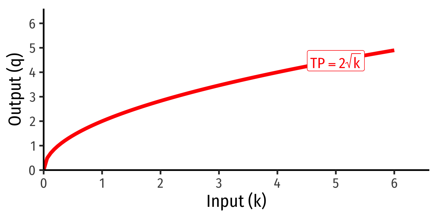
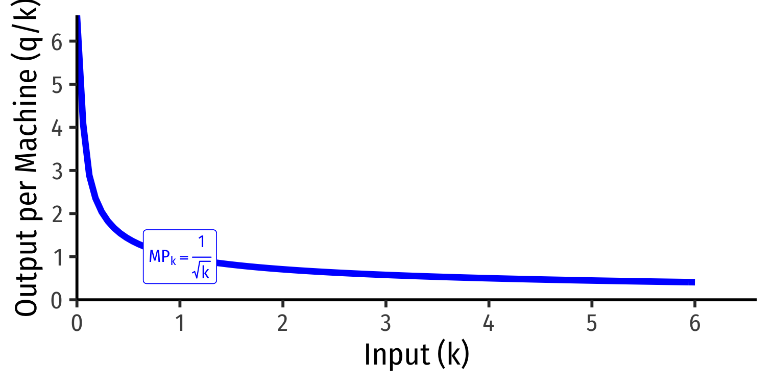
Marginal product of capital (MPk): additional output produced by adding one more unit of capital (holding l constant) MPk=ΔqΔk
MPk is slope of TP at each value of k!
Note: via calculus: ∂q∂k
Note we often don't consider capital in the short run!
Diminishing Returns
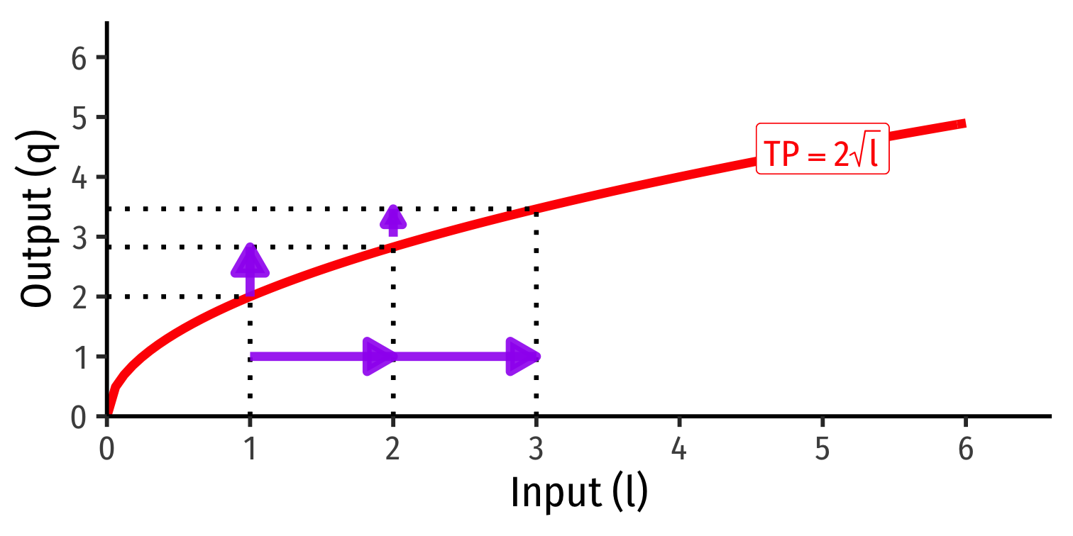
Law of Diminishing Returns: adding more of one factor of production holding all others constant will result in successively lower increases in output
In order to increase output, firm will need to increase all factors!

Diminishing Returns
Law of Diminishing Returns: adding more of one factor of production holding all others constant will result in successively lower increases in output
In order to increase output, firm will need to increase all factors!

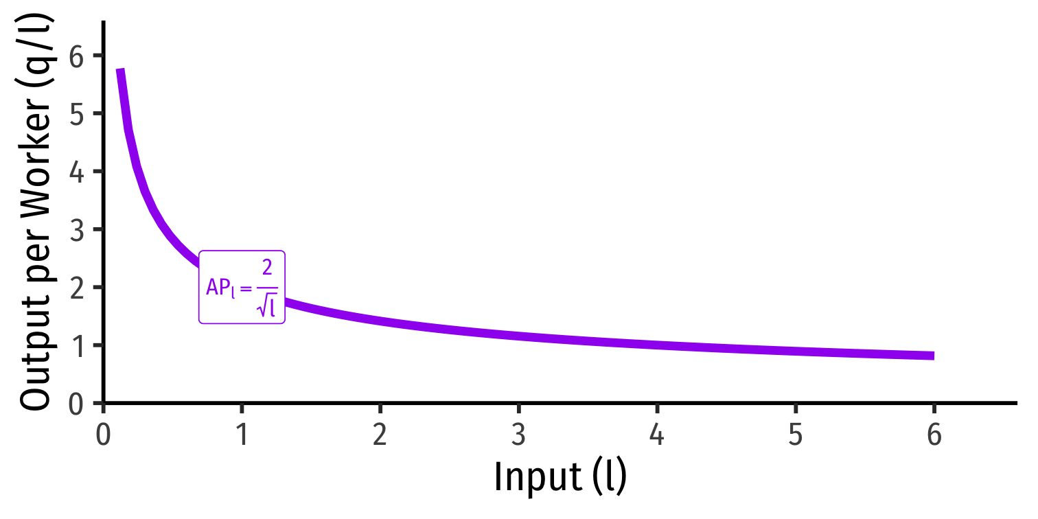
Average Product of Labor (and Capital)
Average product of labor (APl): total output per worker APl=ql
A measure of labor productivity
Average product of capital (APk): total output per unit of capital APk=qk

The Long Run
- In the long run, all factors of production are variable
q=f(k,l)
Can build more factories, open more storefronts, rent more space, invest in machines, etc.
So the firm can choose both l and k

The Firm's Problem
Based on what we've discussed, we can fill in a constrained optimization model for the firm
- But don't write this one down just yet!
The firm's problem is:
Choose: < inputs and output >
In order to maximize: < profits >
Subject to: < technology >
- It's actually much easier to break this into 2 stages, though it's possible to do it all at once. See today's class notes page for an example.

The Firm's Two Problems
- 1st Stage: firm's profit maximization problem:
Choose: < output >
In order to maximize: < profits >
- We'll cover this later...first we'll explore:
The Firm's Two Problems
- 1st Stage: firm's profit maximization problem:
Choose: < output >
In order to maximize: < profits >
We'll cover this later...first we'll explore:
2nd Stage: firm's cost minimization problem:
Choose: < inputs >
In order to minimize: < cost >
Subject to: < producing the optimal output >
- Minimizing costs ⟺ maximizing profits
Mapping Input-Combination Choices Graphically
3-D Production Function
2-D Isoquant Contours
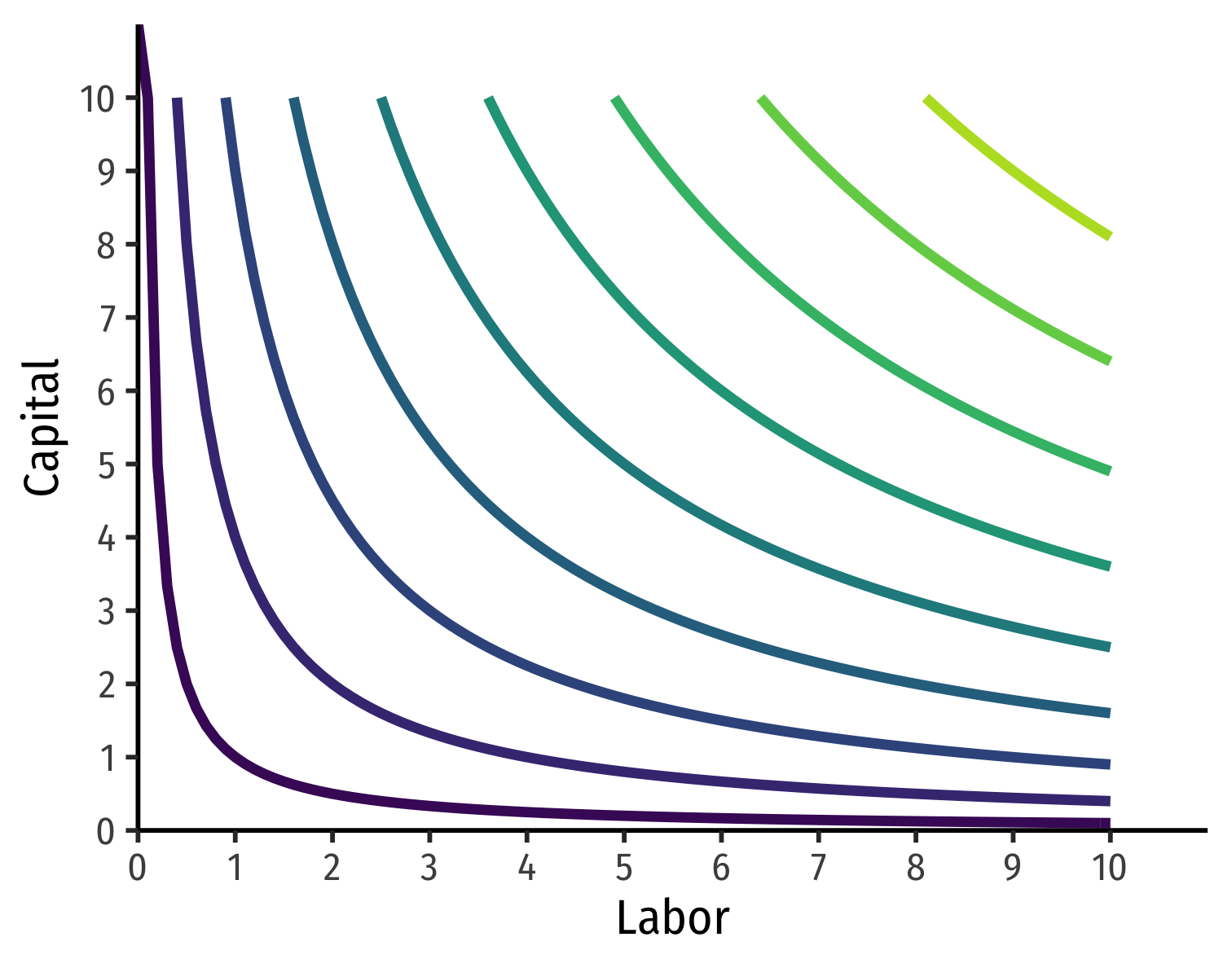
Isoquant Curves
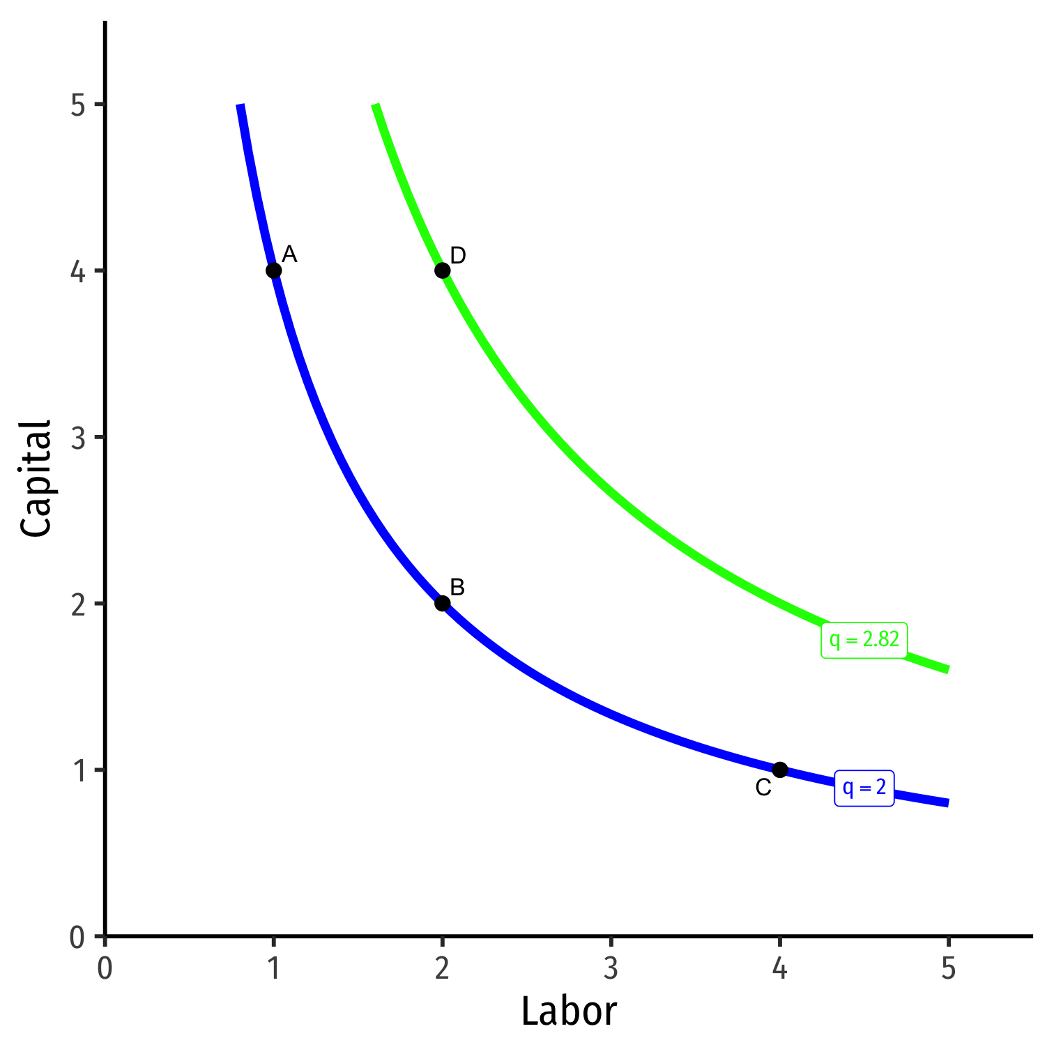
- We can draw an isoquant indicating all combinations of l and k that yield the same q
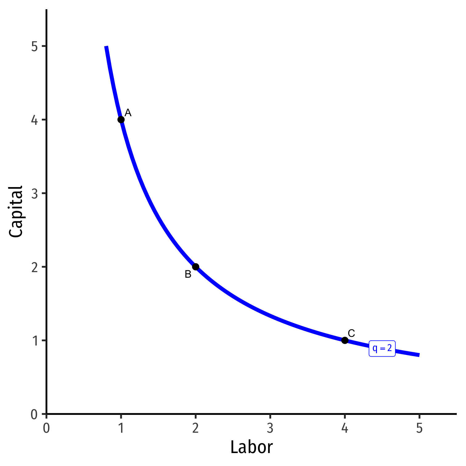
Isoquant Curves
We can draw an isoquant indicating all combinations of l and k that yield the same q
Combinations above curve yield more output; on a higher curve
- D>A=B=C
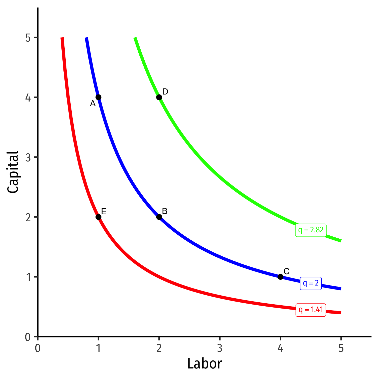
Isoquant Curves
We can draw an isoquant indicating all combinations of l and k that yield the same q
Combinations above curve yield more output; on a higher curve
- D>A=B=C
Combinations below the curve yield less output; on a lower curve
- E<A=B=C
Marginal Rate of Technical Substitution I
- If your firm uses fewer workers, how much more capital would it need to produce the same amount?

Marginal Rate of Technical Substitution I
If your firm uses fewer workers, how much more capital would it need to produce the same amount?
Marginal Rate of Technical Substitution (MRTS): rate at which firm trades off one input for another to yield the same output
Marginal Rate of Technical Substitution I
Think of this as the opportunity cost: # of units of k you need to give up to acquire 1 more l
MRTS measures firm's tradeoff between l and k based on its technology
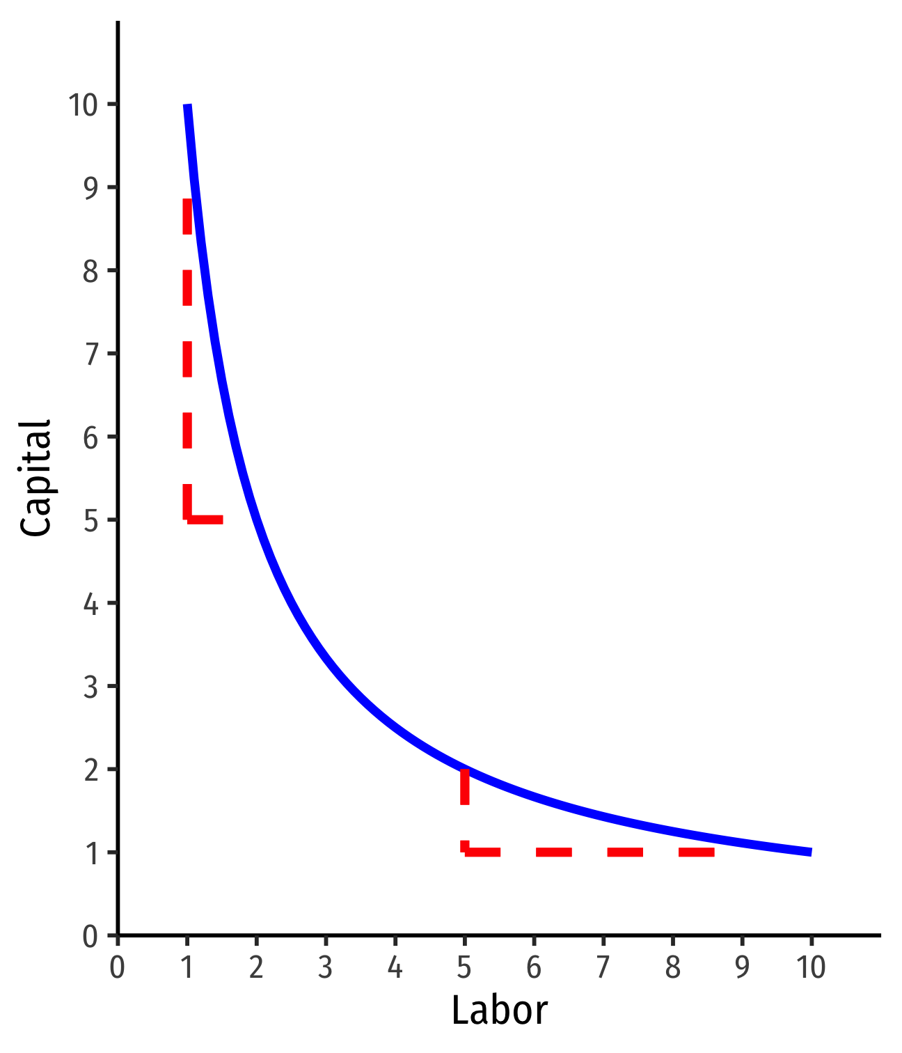
Marginal Rate of Technical Substitution II
MRTS is the slope of the isoquant MRTSl,k=−ΔkΔl=riserun
Amount of k given up for 1 more l
Note: slope (MRTS) changes along the curve!
Law of diminishing returns!
MRTS and Marginal Products
- Relationship between MP and MRTS:
ΔkΔl⏟MRTS=−MPlMPk
See proof in today's class notes
Sound familiar? 🧐

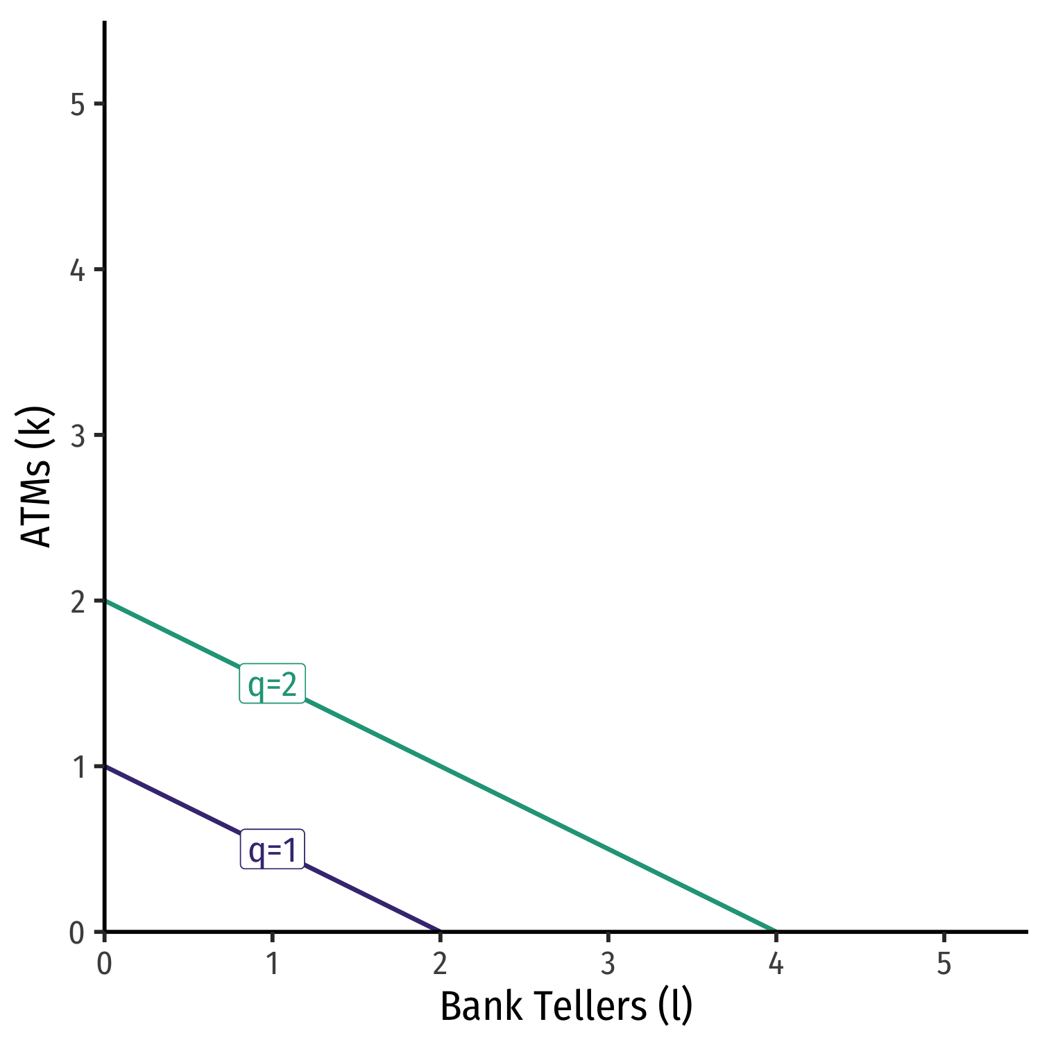
Special Case I: Perfect Substitutes
Example: Consider Bank Tellers (l) and ATMs (k)
One ATM can do the work of 2 bank tellers
Perfect substitutes: inputs that can be substituted at same fixed rate and yield same output
MRTSl,k=−0.5 (a constant!)
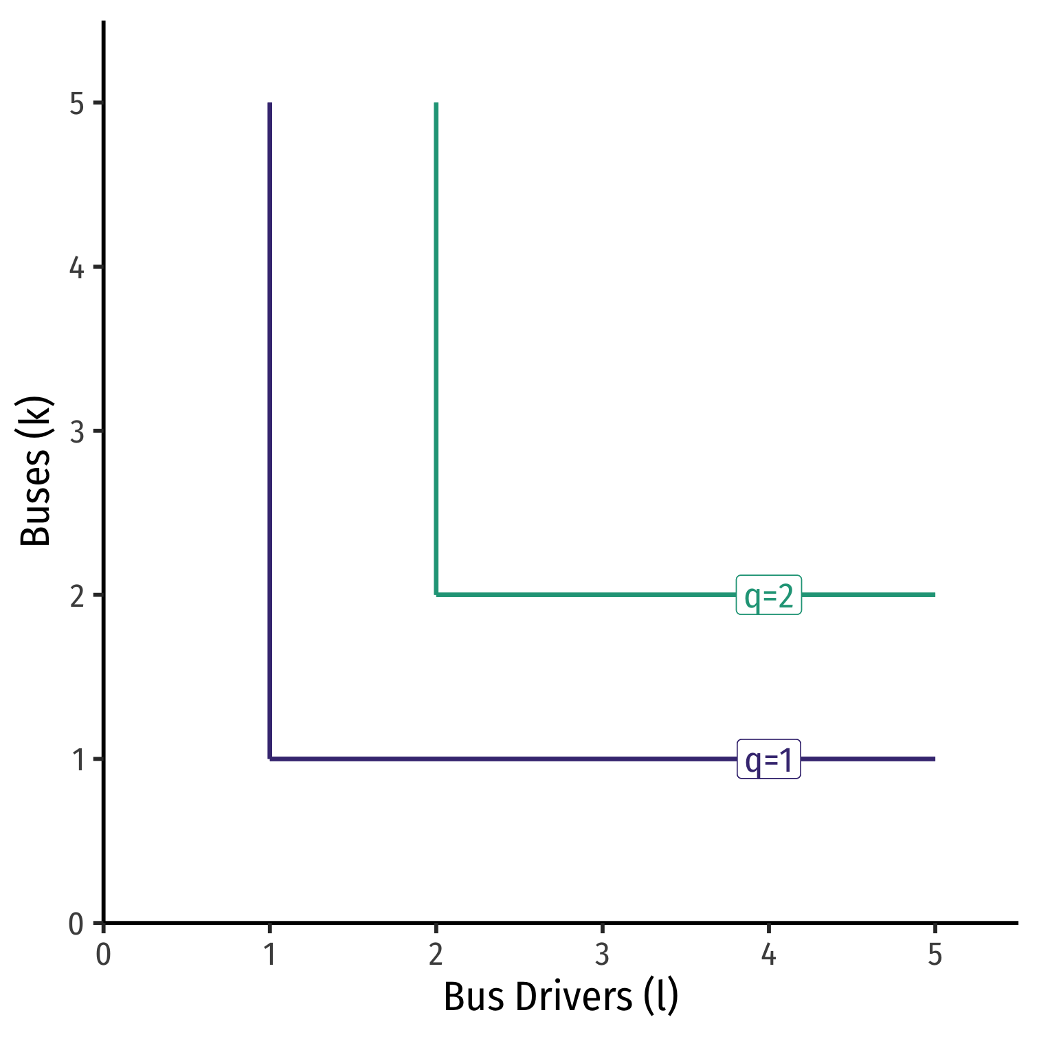
Special Case II: Perfect Complements
Example: Consider busses (k) and bus drivers (l)
Must combine together in fixed proportions (1:1)
Perfect complements: inputs must be used together in same fixed proportion to produce output
MRS: ?
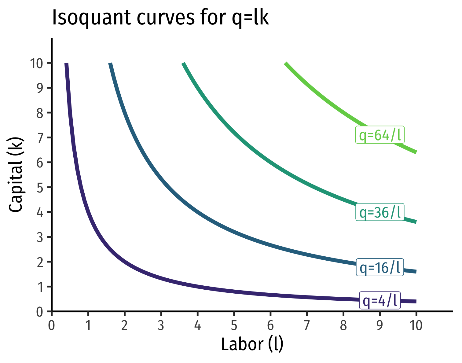
Common Case: Cobb-Douglas Production Functions
- Again: very common functional form in economics is Cobb-Douglas
q=Akalb
Where a,b>0 (and very often a+b=1)
A is total factor productivity
Isocost Lines
If your firm can choose among many input combinations to produce q, which combinations are optimal?
Those combination that are cheapest
Denote prices of each input as:
- w: price of labor (wage)
- r: price of capital
Let C be the total cost of using inputs (l,k) at current input prices (w,r) to produce q units of output:
C(w,r,q)=wl+rk

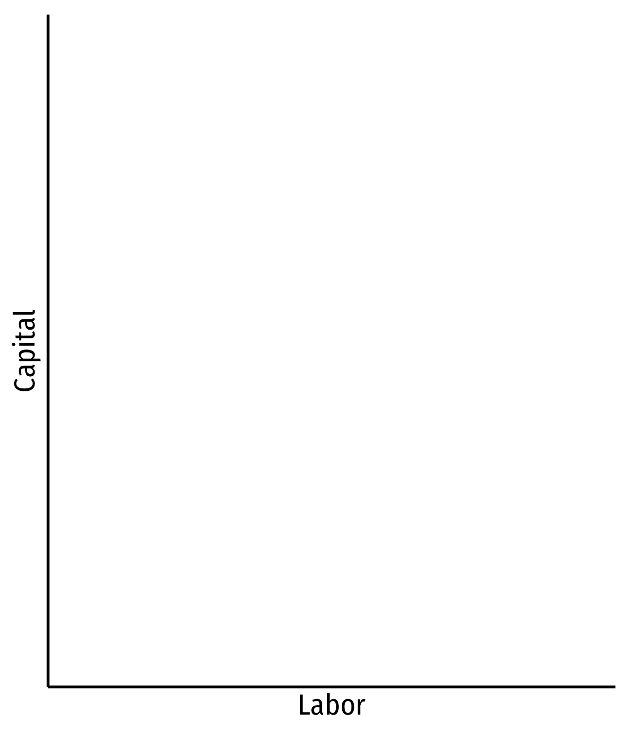
The Isocost Line, Graphically
wl+rk=C
- Solve for k to graph
k=Cr−wrl
The Isocost Line, Graphically
wl+rk=C
- Solve for k to graph
k=Cr−wrl
- Vertical-intercept: Cr
- Horizontal-intercept: Cw
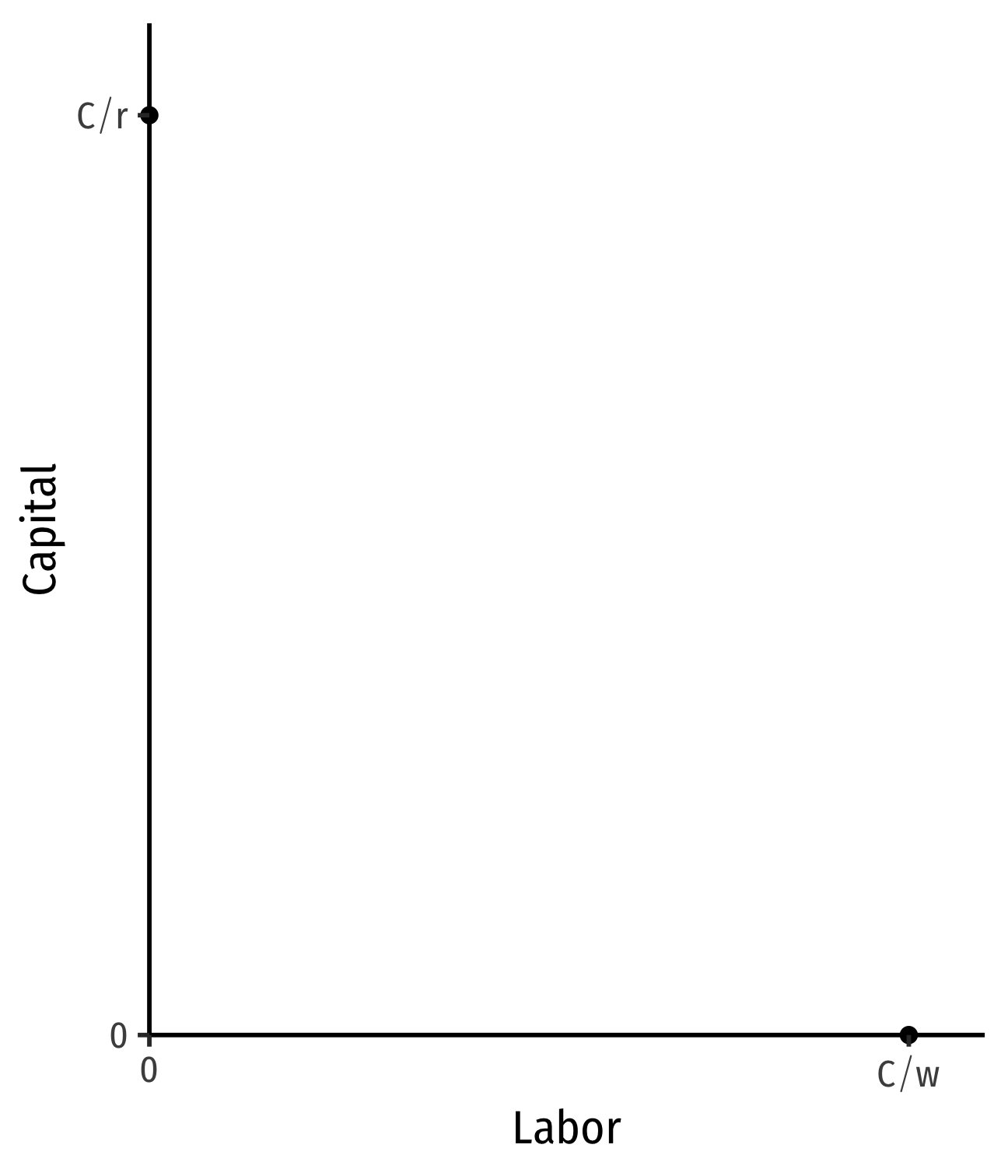
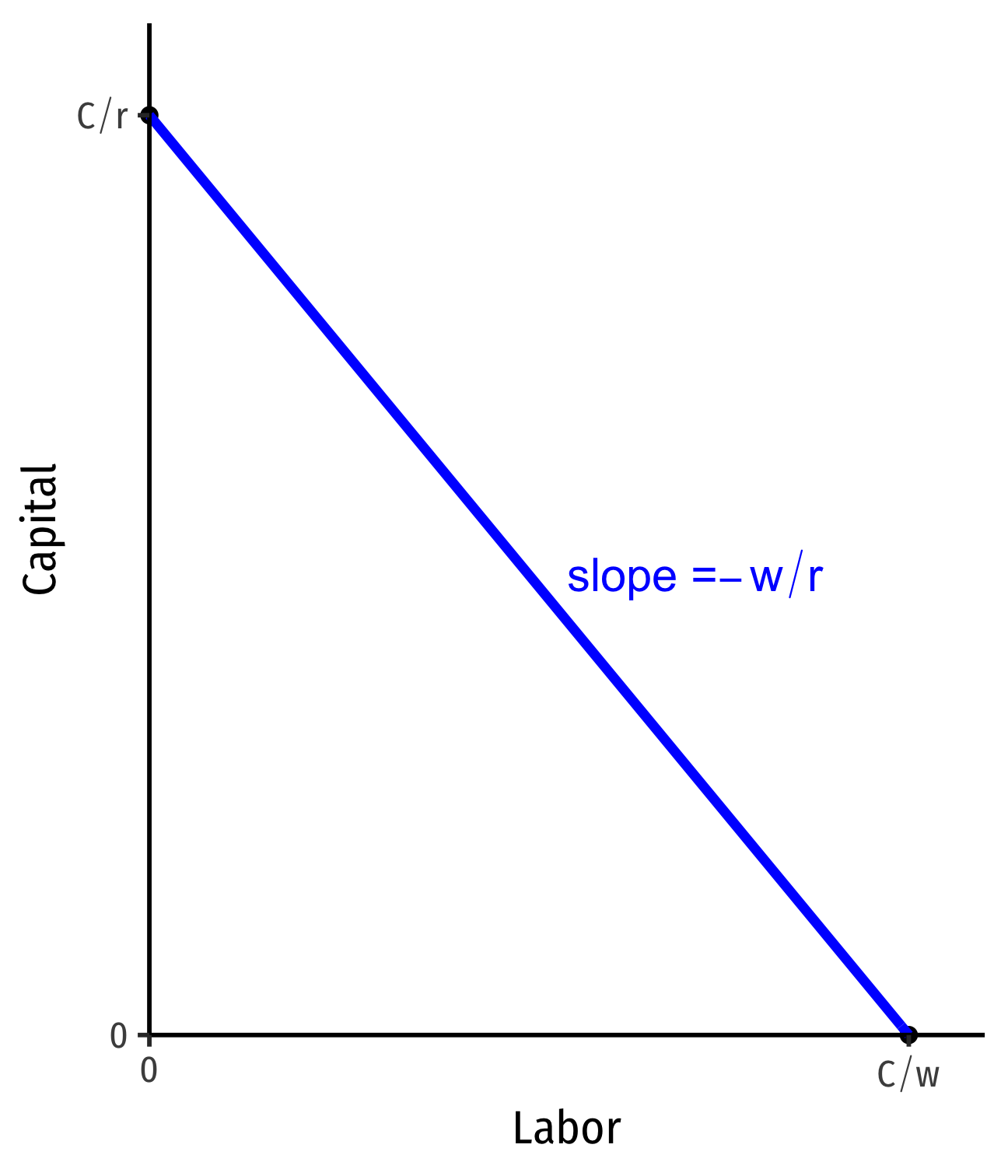
The Isocost Line, Graphically
wl+rk=C
- Solve for k to graph
k=Cr−wrl
- Vertical-intercept: Cr
- Horizontal-intercept: Cw
- slope: −wr

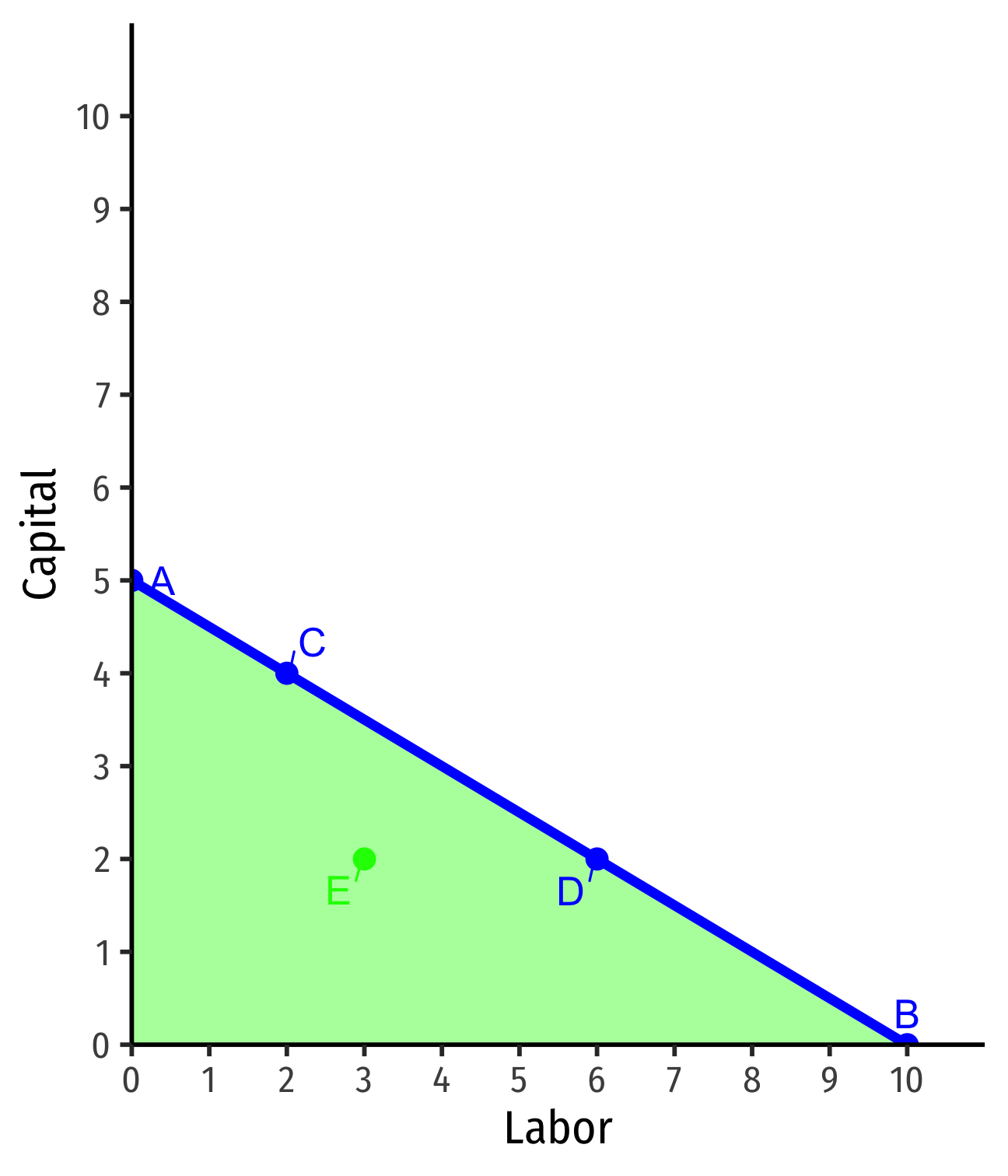
Interpreting Isocost Line
- Points on the line are same total cost
- A: $5(0l)+$10(5k)=$50
- B: $5(10l)+$10(0k)=$50
- C: $5(2l)+$10(4k)=$50
- D: $5(6l)+$10(2k)=$50

Interpreting Isocost Line
Points on the line are same total cost
- A: $5(0l)+$10(5k)=$50
- B: $5(10l)+$10(0k)=$50
- C: $5(2l)+$10(4k)=$50
- D: $5(6l)+$10(2k)=$50
Points beneath the line are cheaper (but may produce less)
- E: $5(3l)+$10(2k)=$35
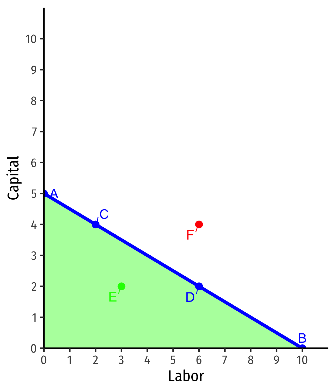
Interpreting the Isocost Line
Points on the line are same total cost
- A: $5(0l)+$10(5k)=$50
- B: $5(10l)+$10(0k)=$50
- C: $5(2l)+$10(4k)=$50
- D: $5(6l)+$10(2k)=$50
Points beneath the line are cheaper (but may produce less)
- E: $5(3l)+$10(2k)=$35
Points above the line are more expensive (and may produce more)
- F: $5(6l)+$10(4k)=$70
Interpretting the Slope
Slope: market-rate of tradeoff between l and k
Relative price of l or opportunity cost of l:
Using 1 more unit of l requires giving up wr units of k
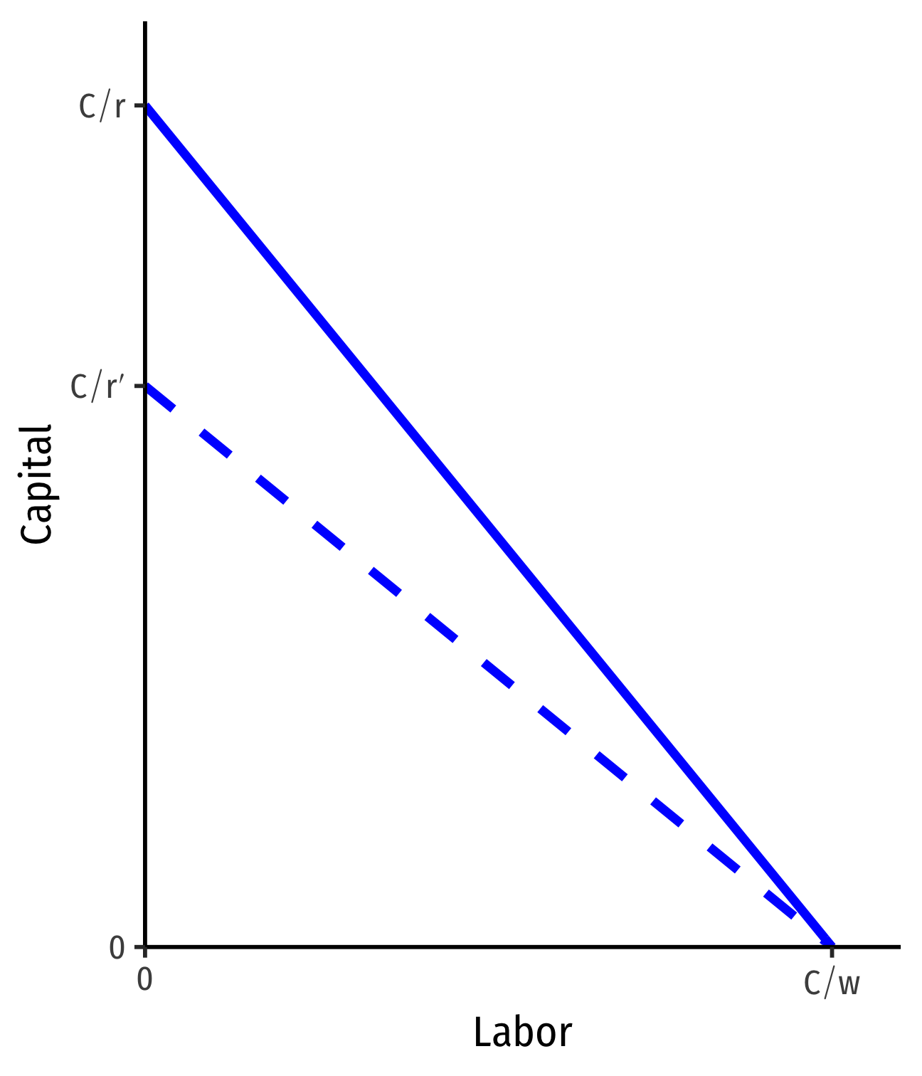
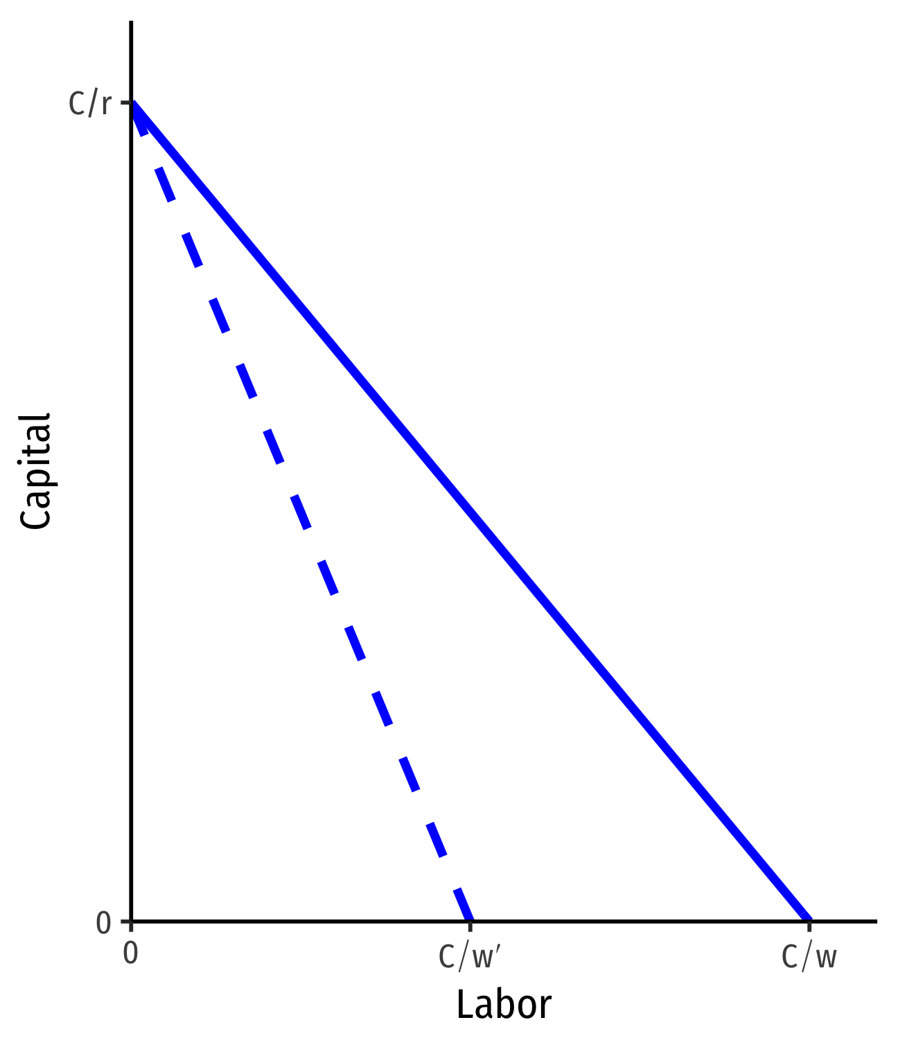
Changes in Relative Factor Prices I
- Changes in relative factor prices: rotate the line
Example: An increase in the price of l
- Slope changes: −w′r

Changes in Relative Factor Prices II
- Changes in relative factor prices: rotate the line
Example: An increase in the price of k
- Slope changes: −wr′