2.3 — Cost Minimization
ECON 306 · Microeconomic Analysis · Fall 2020
Ryan Safner
Assistant Professor of Economics
safner@hood.edu
ryansafner/microF20
microF20.classes.ryansafner.com
Recall: The Firm's Two Problems
- 1st Stage: firm's profit maximization problem:
Choose: < output >
In order to maximize: < profits >
We'll cover this later...first we'll explore:
2nd Stage: firm's cost minimization problem:
Choose: < inputs >
In order to minimize: < cost >
Subject to: < producing the optimal output >
- Minimizing costs ⟺ maximizing profits

Solving the Cost Minimization Problem
The Firm's Cost Minimization Problem
- The firm's cost minimization problem is:
Choose: < inputs: l,k>
In order to maximize: < total cost: wl+rk >
Subject to: < producing the optimal output: q∗=f(l,k) >

The Cost Minimization Problem: Tools
Our tools for firm's input choices:
Choice: combination of inputs (l,k)
Production function/isoquants: firm's technological constraints
- How the firm trades off between inputs
- Isocost line: firm's total cost (for given output and input prices)
- How the market trades off between inputs

The Cost Minimization Problem: Verbally
- The firms's cost minimization problem:
choose a combination of l and k to minimize total cost that produces the optimal amount of output

The Cost Minimization Problem: Math
minl,kwl+rk
- This requires calculus to solve. We will look at graphs instead!

The Firm's Least-Cost Input Combination: Graphically
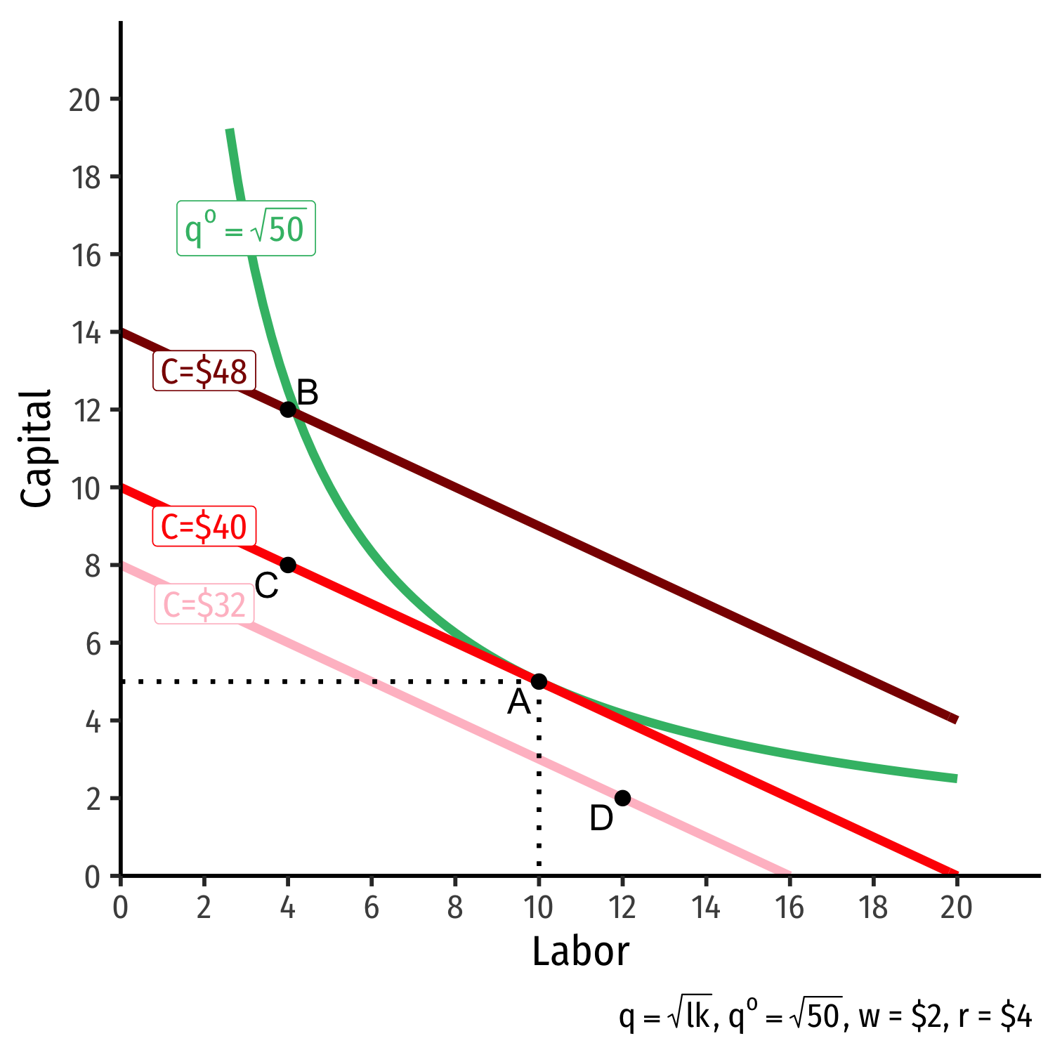
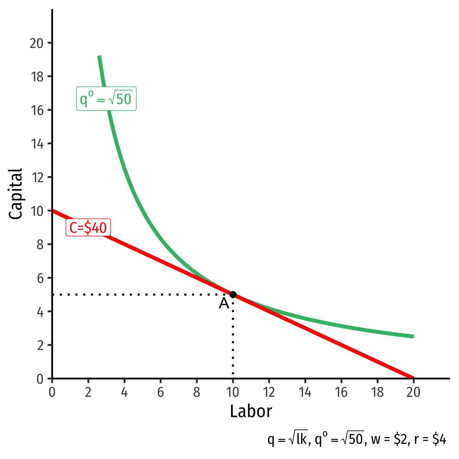
- Graphical solution: Lowest isocost line tangent to desired isoquant (A)

The Firm's Least-Cost Input Combination: Graphically
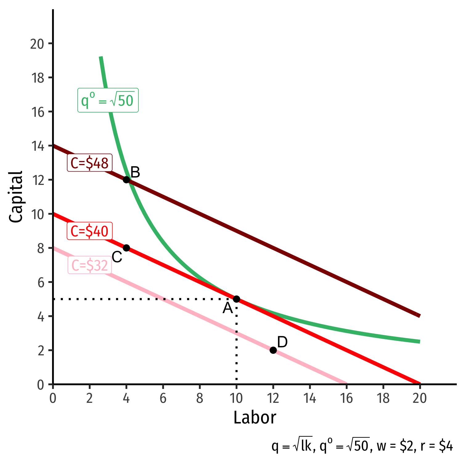
Graphical solution: Lowest isocost line tangent to desired isoquant (A)
B produces same output as A, but higher cost
C is same cost as A, but produces less than desired output
D produces is cheaper, but produces less than desired output

The Firm's Least-Cost Input Combination: Why A?
Isoquant curve slope=Isocost line slope

The Firm's Least-Cost Input Combination: Why A?
Isoquant curve slope=Isocost line slope|MRTSl,k|=|wr||MPlMPk|=|wr||−0.5|=|−0.5|
Firm would exchange at same rate as market
No other combination of (l,k) exists at current prices & output that could lower cost to produce q∗!

Two Equivalent Rules
Rule 1
MPlMPk=wr
- Easier for solving math problems

Two Equivalent Rules
Rule 1
MPlMPk=wr
- Easier for solving math problems
Rule 2
MPlw=MPkr
- Easier for intuition (next slide)

The Equimarginal Rule Again I
MPlw=MPkr=⋯=MPnpn
Equimarginal Rule: the cost of production is minimized where the marginal product per dollar spent is equalized across all n possible inputs
Firm will always choose an option that gives higher marginal product (e.g. if MPl>MPk)
- But each option has a different cost, so we weight each option by its cost, hence MPnpn
The Equimarginal Rule Again II
MPlw=MPkr=⋯=MPnpn
Why is this the optimum?
Example: suppose firm could get a higher marginal product per $1 spent on l than for k (i.e. "more bang for your buck"!)
- Not minimizing costs!
- Should use more l and less k!
- This will raise MPk and lower MPl!
- Continue until cost-adjusted marginal products are equalized
The Equimarginal Rule Again III
Any optimum in economics: no better alternatives exist under current constraints
No possible change in your inputs to produce q∗ that would lower cost

The Firm's Least-Cost Input Combination: Example
Example:
Your firm can use labor l and capital k to produce output according to the production function: q=2lk
The marginal products are:
MPl=2kMPk=2l
You want to produce 100 units, the price of labor is $10, and the price of capital is $5.
- What is the least-cost combination of labor and capital that produces 100 units of output?
- How much does this combination cost?
Returns to Scale
Returns to Scale
- The returns to scale of production refers to the change in output when all inputs are increased at the same rate
Returns to Scale
The returns to scale of production refers to the change in output when all inputs are increased at the same rate
Constant returns to scale: output increases at same proportionate rate as inputs increase
- e.g. if you double all inputs, output doubles
Returns to Scale
The returns to scale of production refers to the change in output when all inputs are increased at the same rate
Constant returns to scale: output increases at same proportionate rate as inputs increase
- e.g. if you double all inputs, output doubles
- Increasing returns to scale: output increases more than proportionately to the change in inputs
- e.g. if you double all inputs, output more than doubles
- Decreasing returns to scale: output increases less than proportionately to the change in inputs
- e.g. if you double all inputs, output less than doubles
Returns to Scale: Example
Example: Does each of the following production functions exhibit constant returns to scale, increasing returns to scale, or decreasing returns to scale?
q=4l+2k
q=2lk
q=2l0.3k0.3
Returns to Scale: Cobb-Douglas
One reason we often use Cobb-Douglas production functions is to easily determine returns to scale:
q=Akαlβα+β=1: constant returns to scale
- α+β>1: increasing returns to scale
- α+β<1: decreasing returns to scale
- Note this trick only works for Cobb-Douglas functions!
Cobb-Douglas: Constant Returns Case
In the constant returns to scale case (most common), Cobb-Douglas is often written as:
q=Akαl1−αα is the output elasticity of capital
- A 1% increase in k leads to a α% increase in q
1−α is the output elasticity of labor
- A 1% increase in l leads to a (1−α)% increase in q
Output-Expansion Paths & Cost Curves

Goolsbee et. al (2011: 246)
Output Expansion Path: curve illustrating the changes in the optimal mix of inputs and the total cost to produce an increasing amount of output
Total Cost curve: curve showing the total cost of producing different amounts of output (next class)
See next class' notes page to see how we go from our least-cost combinations over a range of outputs to derive a total cost function