Recall: The Firm's Two Problems
- 1st Stage: firm's profit maximization problem:
Choose: < output >
In order to maximize: < profits >
We'll cover this later...first we'll explore:
2nd Stage: firm's cost minimization problem:
Choose: < inputs >
In order to minimize: < cost >
Subject to: < producing the optimal output >
- Minimizing costs ⟺ maximizing profits

A Competitive Market
- We assume (for now) the firm is in a competitive industry:
Firms’ products are perfect substitutes
Firms are “price-takers”, no one firm can affect the market price
Market entry and exit are free†
† Remember this feature. It turns out to be the most important feature that distinguishes different types of industries!
Profit
Recall that profit is is: π=pq⏟revenues−(wl+rk)⏟costs
We’ll first take a closer look at costs today, then at revenues
Next class we'll put them together to find q∗ that maximizes π (the first stage problem)
Costs in Economics are Opportunity Costs
- Remember, economic costs are different from common conception of "cost"
- Accounting cost: monetary cost
- Economic cost: value of next best alternative use of resources given up (i.e. opportunity cost)


Costs in Economics are Opportunity Costs
This leads to the difference between
- Accounting profit: revenues minus accounting costs
- Economic profit: revenues minues opportunity costs
One of the most difficult concepts to think about!
Costs in Economics are Opportunity Costs
Another helpful perspective:
Accounting cost: what you historically paid for a resource
Economic cost: what you can currently get in the market for a selling a resource
- Resource's value in alternative uses
Costs in Economics are Opportunity Costs
Because resources are scarce, and have rivalrous uses,
In functioning markets, the market price measures the opportunity cost of using a resource for an alternative use
Firms not only pay for direct use of a resource, but also indirectly for "pulling it out" of an alternate use in the economy!
Opportunity Costs in Production
- Every choice incurs an opportunity cost
Examples:
- If you choose to start a business, you may give up your salary at your current job
- If you invest in a factory, you give up other investment opportunities
- If you use an office building you own, you cannot rent it to other people
- If you hire a skilled worker, you must pay them a high enough salary to deter them from working for other firms
Opportunity Cost is Hard for People

Opportunity Costs vs. Sunk Costs
Opportunity cost is a forward-looking concept
Choices made in the past with non-recoverable costs are called sunk costs
Sunk costs should not enter into future decisions
Many people have difficulty letting go of unchangeable past decisions: sunk cost fallacy

Sunk Costs: Examples

Sunk Costs: Examples

Sunks Costs: Examples

The Sunk Cost Fallacy

Common Sunk Costs in Business
Licensing fees, long-term lease contracts
Specific capital (with no alternative use): uniforms, menus, signs
Research & Development spending
Advertising spending
The Accounting vs. Economic Point of View I
- Helpful to consider two points of view:
"Accounting point of view": are you taking in more cash than you are spending?
"Economic point of view": is your product you making the best social use of your resources (i.e. are there higher-valued uses of your resources you are keeping them away from)?
The Accounting vs. Economic Point of View II
Social implications: are consumers best off with you using scarce resources (with alternative uses!) to produce your current product?
Remember: this is an economics course, not a business course!
- What might be good/bad for one business might have bad/good consequences for society!
- e.g. monopoly vs. competition
Fixed vs. Variable costs: Examples

Example: Airlines
Fixed costs: the aicraft
Variable costs: getting one more customer in a seat
Fixed vs. Variable costs: Examples

Example: Car Factory
Fixed costs: the factory, machines in the factory
Variable costs: producing one more car
Fixed vs. Variable costs: Examples

Example: Starbucks
Fixed costs: the retail space
Variable costs: producing one more cup of coffee
Fixed vs. Sunk costs
Diff. between fixed vs. sunk costs?
Sunk costs are a type of fixed cost that are not avoidable or recoverable
Many fixed costs can be avoided or changed in the long run
Common fixed, but not sunk, costs:
- rent for office space, durable equipment, operating permits (that are renewed)
When deciding to stay in business, fixed costs matter, sunk costs do not!
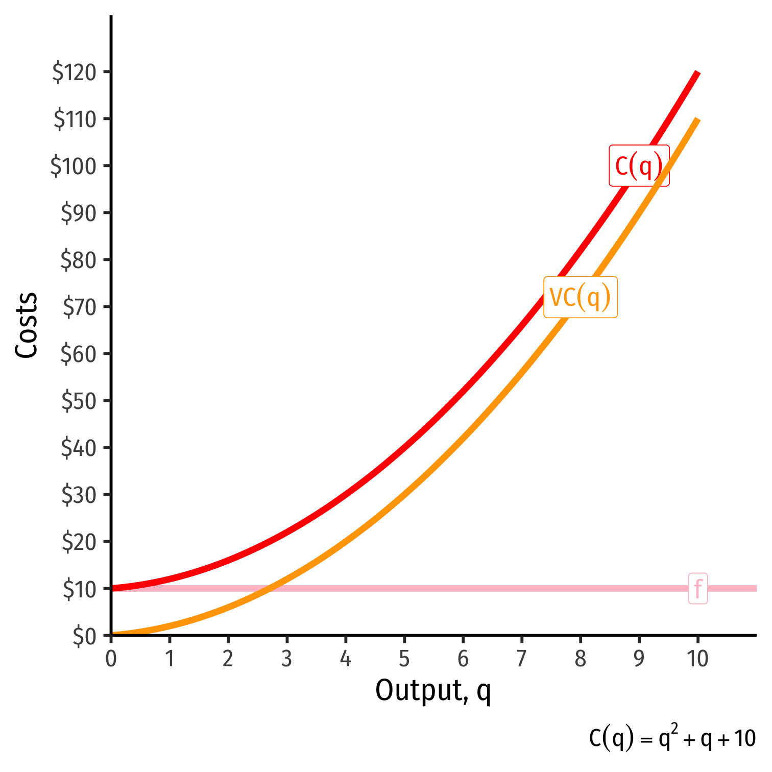
Cost Functions: Example, Visualized
| q | f | VC(q) | C(q) |
|---|---|---|---|
| 0 | 10 | 0 | 10 |
| 1 | 10 | 2 | 12 |
| 2 | 10 | 6 | 16 |
| 3 | 10 | 12 | 22 |
| 4 | 10 | 20 | 30 |
| 5 | 10 | 30 | 40 |
| 6 | 10 | 42 | 52 |
| 7 | 10 | 56 | 66 |
| 8 | 10 | 72 | 82 |
| 9 | 10 | 90 | 100 |
| 10 | 10 | 110 | 120 |
The Importance of Marginal Cost

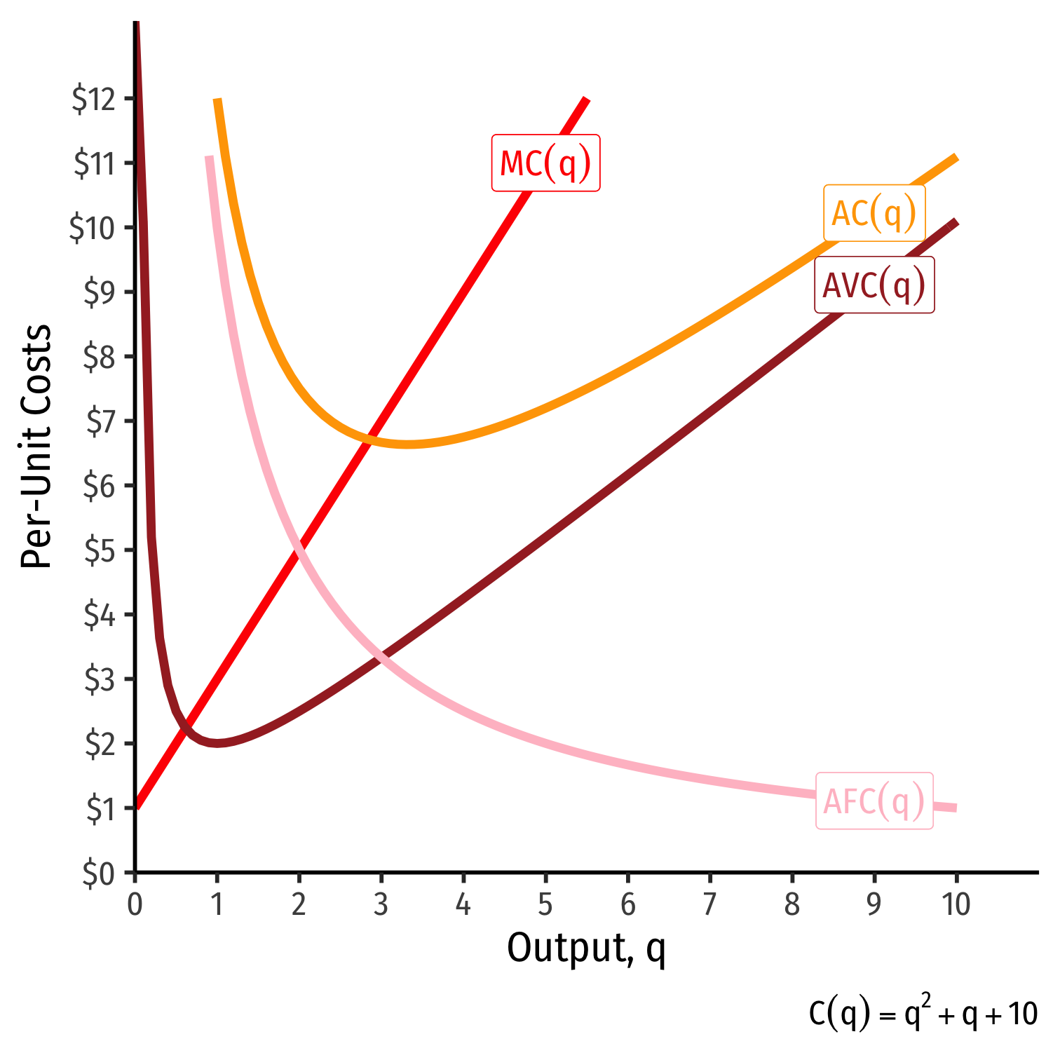
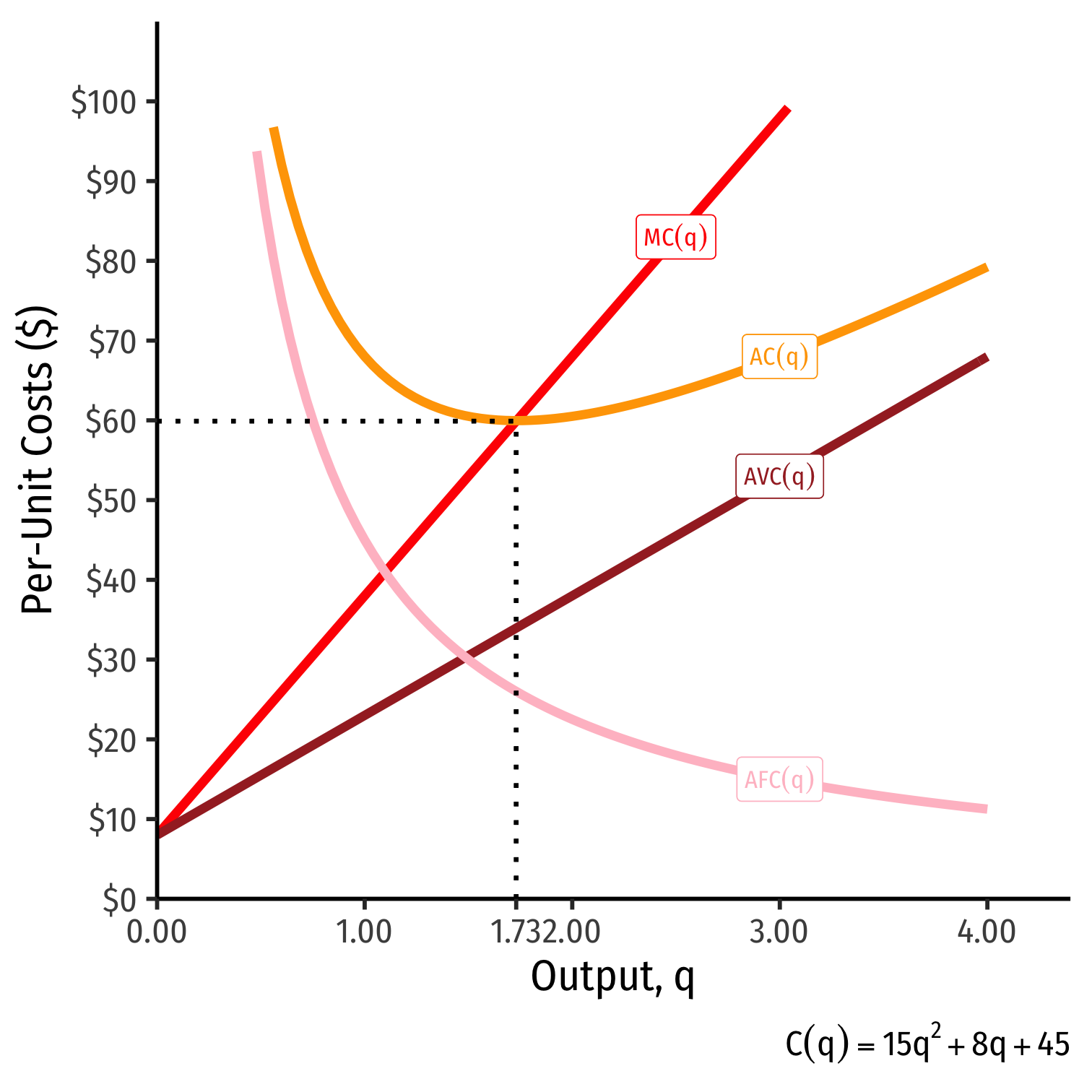
Average and Marginal Costs: Visualized
| q | C(q) | MC(q) | AFC(q) | AVC(q) | AC(q) |
|---|---|---|---|---|---|
| 0 | 10 | − | − | − | − |
| 1 | 12 | 2 | 10.00 | 2 | 12.00 |
| 2 | 16 | 4 | 5.00 | 3 | 8.00 |
| 3 | 22 | 6 | 3.33 | 4 | 7.30 |
| 4 | 30 | 8 | 2.50 | 5 | 7.50 |
| 5 | 40 | 10 | 2.00 | 6 | 8.00 |
| 6 | 52 | 12 | 1.67 | 7 | 8.70 |
| 7 | 66 | 14 | 1.43 | 8 | 9.40 |
| 8 | 82 | 16 | 1.25 | 9 | 10.25 |
| 9 | 100 | 18 | 1.11 | 10 | 11.10 |
| 10 | 120 | 20 | 1.00 | 11 | 12.00 |
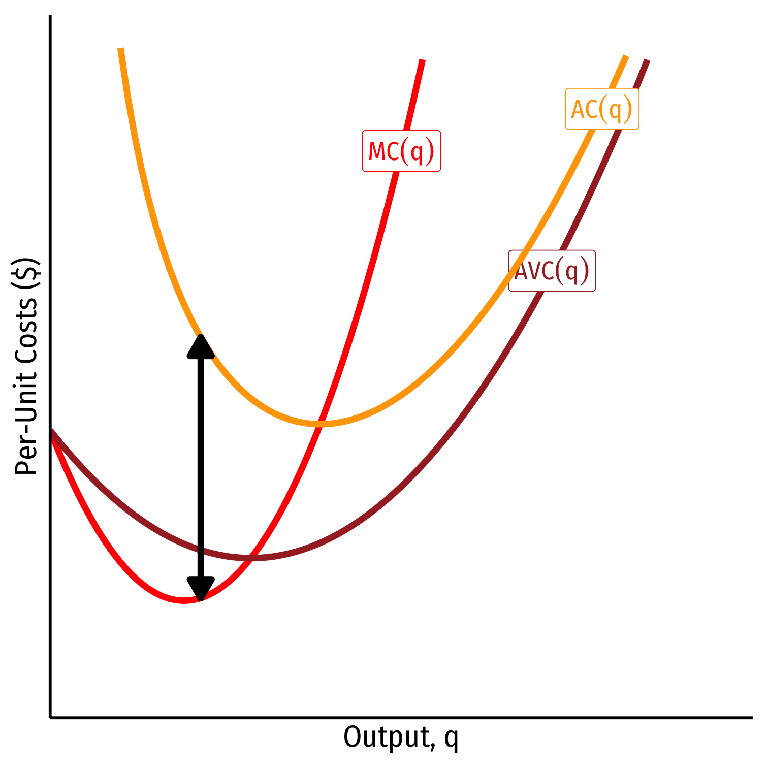
Relationship Between Marginal and Average
Relationship between a marginal and an average value:
marginal > average, average ↑
Relationship Between Marginal and Average
Relationship between a marginal and an average value:
marginal > average, average ↑
marginal < average, average ↓
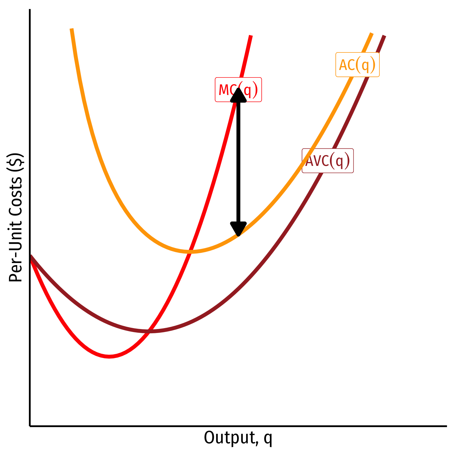
Relationship Between Marginal and Average
Relationship between a marginal and an average value:
marginal > average, average ↑
marginal < average, average ↓
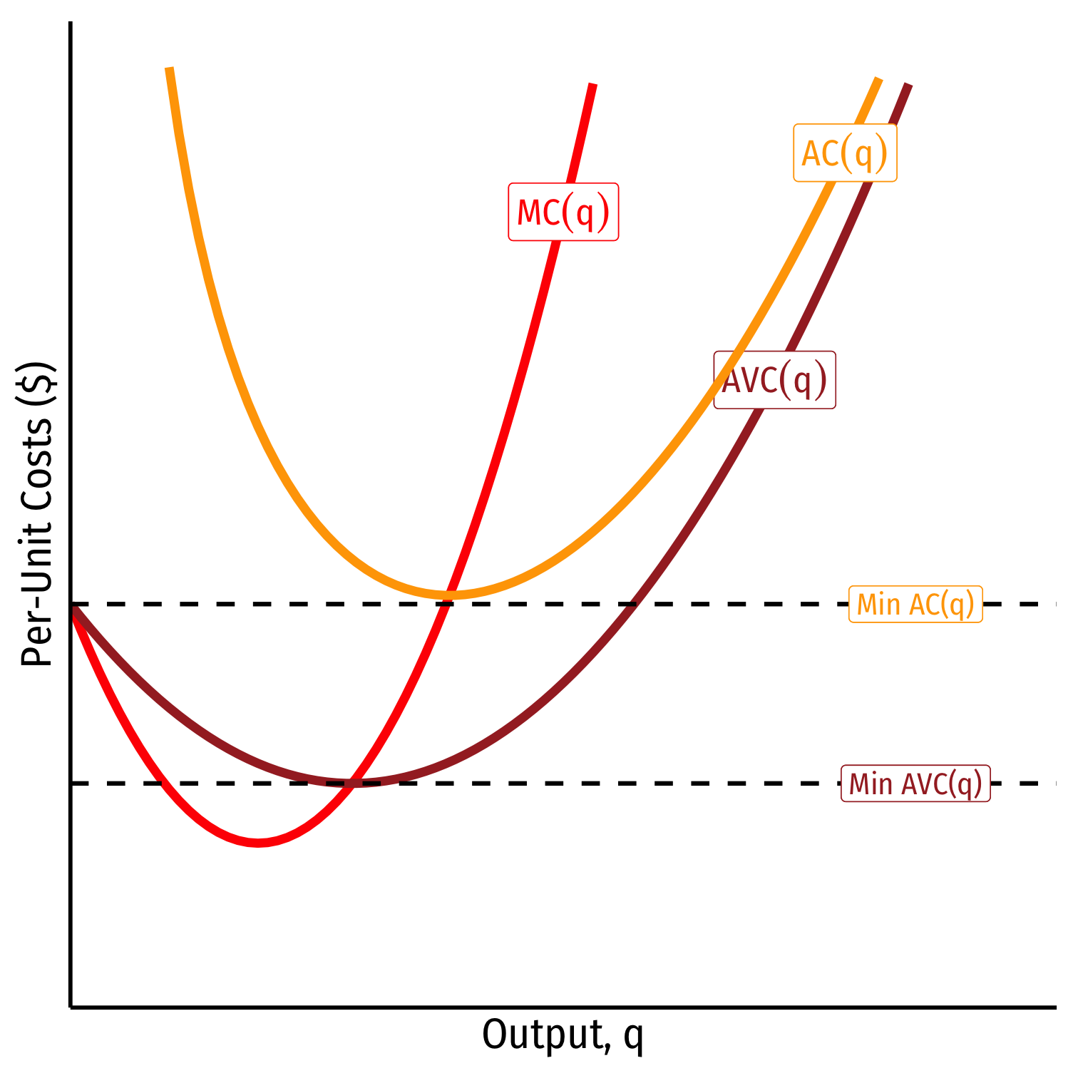
When marginal = average, average is maximized/minimized
- When MC=AC, AC is at a minimum
When MC=AVC, AVC is at a minimum
Economic importance (later): Break-even price and shut-down price
Costs: Example: Visualized
Costs in the Long Run
Long run: firm can change all factors of production & vary scale of production
Long run average cost, LRAC(q): cost per unit of output when the firm can change both l and k to make more q
Long run marginal cost, LRMC(q): change in long run total cost as the firm produce an additional unit of q (by changing both l and/or k)

Average Cost in the Long Run
Long run: firm can choose k (factories, locations, etc)
Separate short run average cost (SRAC) curves for each amount of k potentially chosen
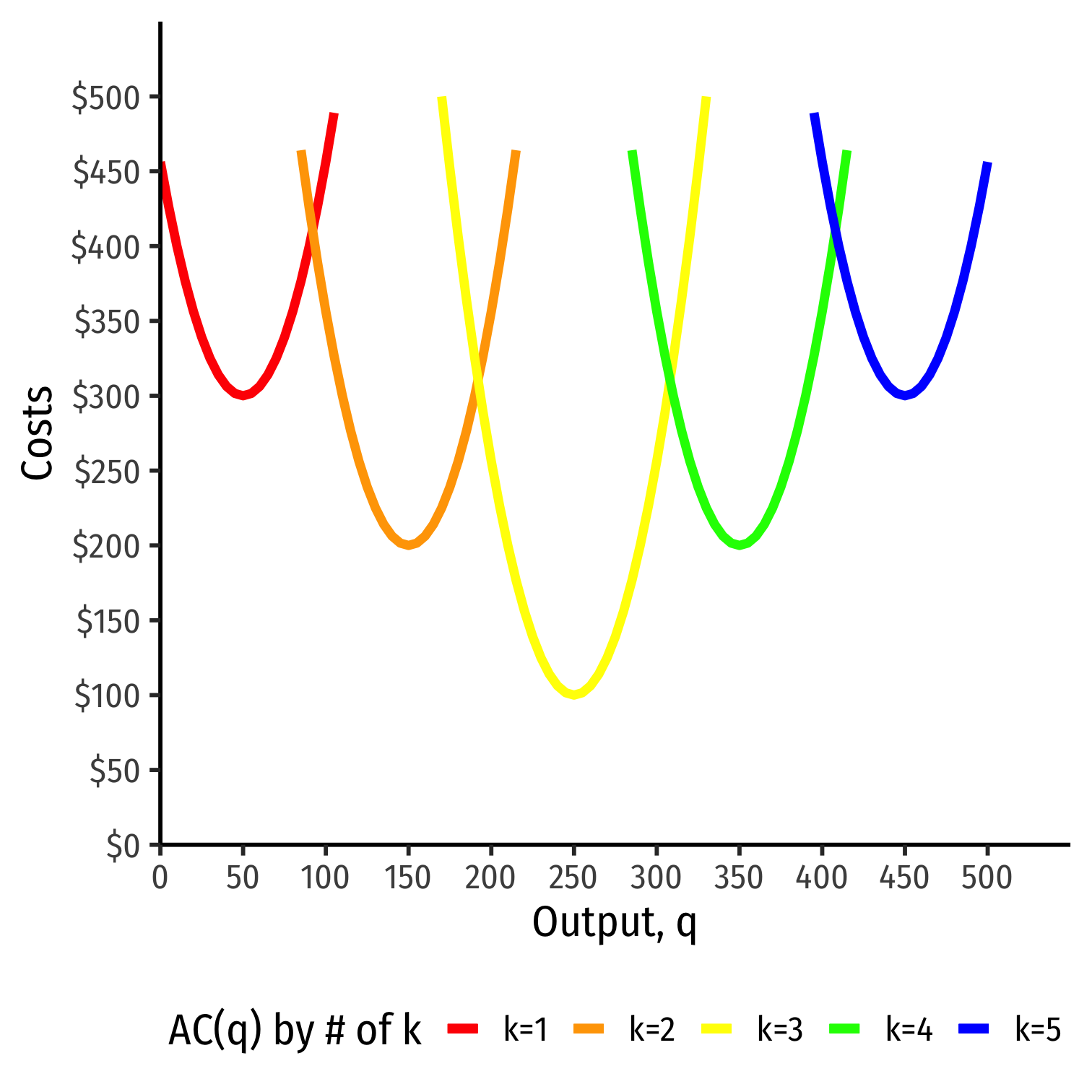
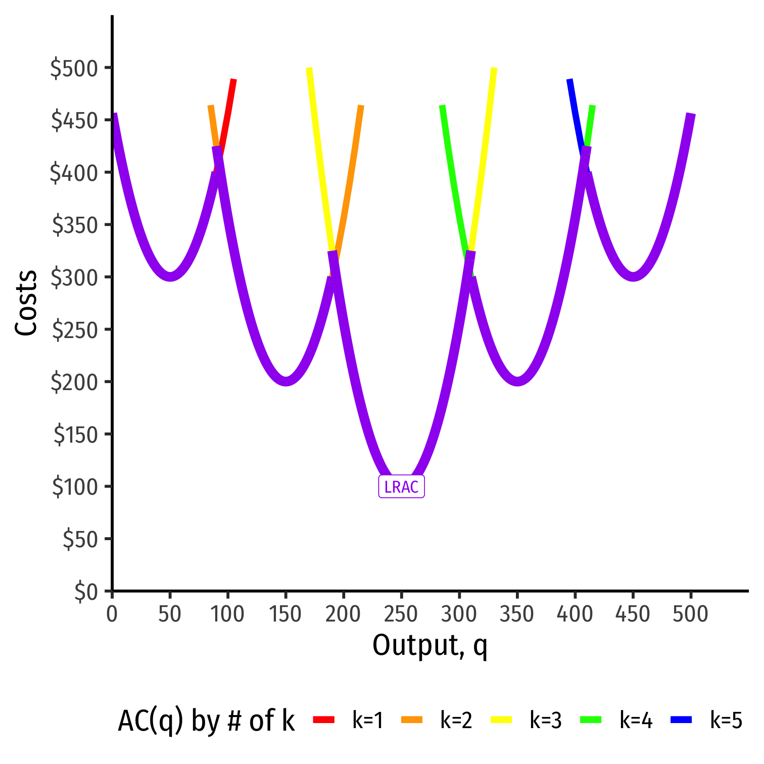
Average Cost in the Long Run
Long run: firm can choose k (factories, locations, etc)
Separate short run average cost (SRAC) curves for each amount of k potentially chosen
Long run average cost (LRAC) curve "envelopes" the lowest (optimal) parts of all the SRAC curves!
"Subject to producing the optimal amount of output, choose l and k to minimize cost"
Long Run Costs & Scale Economies I

Further properties about costs based on scale economies of production:
Economies of scale: costs fall with output
- AFC>AVC(q)
Diseconomies of scale: costs rise with output
- AFC<AVC(q)
Constant economies of scale: costs don't change with output
- Firm at minimum average cost
Long Run Costs & Scale Economies I
Note economies of scale ≠ returns to scale!
Returns to Scale (last class): a technological relationship between inputs & output
Economies of Scale (this class): an economic relationship between output and average costs
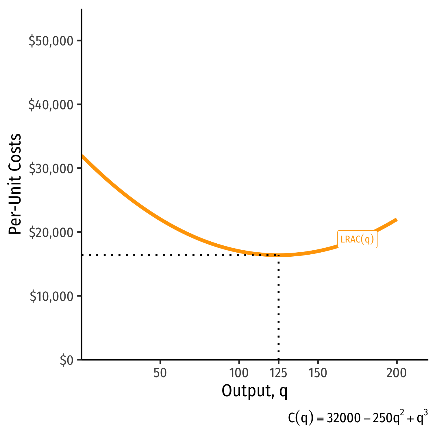
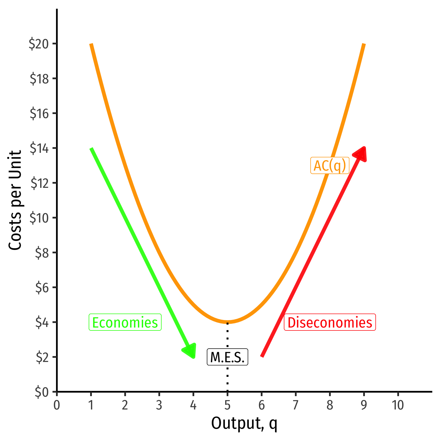
Long Run Costs & Scale Economies II
Minimum Efficient Scale: q with the lowest AC(q)
Economies of Scale: ↑q, ↓AC(q)
Diseconomies of Scale: ↑q, ↑AC(q)
Long Run Costs and Scale Economies: Example