Recall: 2 Major Models of Economics as a “Science”
Optimization
Agents have objectives they value
Agents face constraints
Make tradeoffs to maximize objectives within constraints

Recall: 2 Major Models of Economics as a “Science”
Optimization
Agents have objectives they value
Agents face constraints
Make tradeoffs to maximize objectives within constraints
Equilibrium
Agents compete with others over scarce resources
Agents adjust behaviors based on prices
Stable outcomes when adjustments stop

Recall: Optimization and Equilibrium
If people can learn and change their behavior, they will always switch to a higher-valued option
If there are no alternatives that are better, people are at an optimum
If everyone is at an optimum, the system is in equilibrium


Equilibrium Analysis: Questions to Answer
Where do prices come from?
How do they change?
How consumers and producers to respond to changes?

Equilibrium Analysis
An equilibrium is an allocation of resources such that no individual has an incentive to alter their behavior
In markets: "market-clearing" prices where quantity supplied equals quantity demanded
Partial Equilibrium Analysis
We will only look at "partial equilibrium" in a single market
Changes in one market often affect other markets, affecting the "general equilibrium"
- e.g. a change in the price of corn will affect the market for wheat, soybeans, flax, cereal, sugar, candy, ethanol, gasoline, automobiles, etc...
- think of all of the complements, substitutes, upstream and downstream goods in production...
- General equilibrium is too complicated for undergraduate courses...
Demand Function
- Demand function relates quantity to price
Example: q=10−p
- Not graphable (wrong axes)!

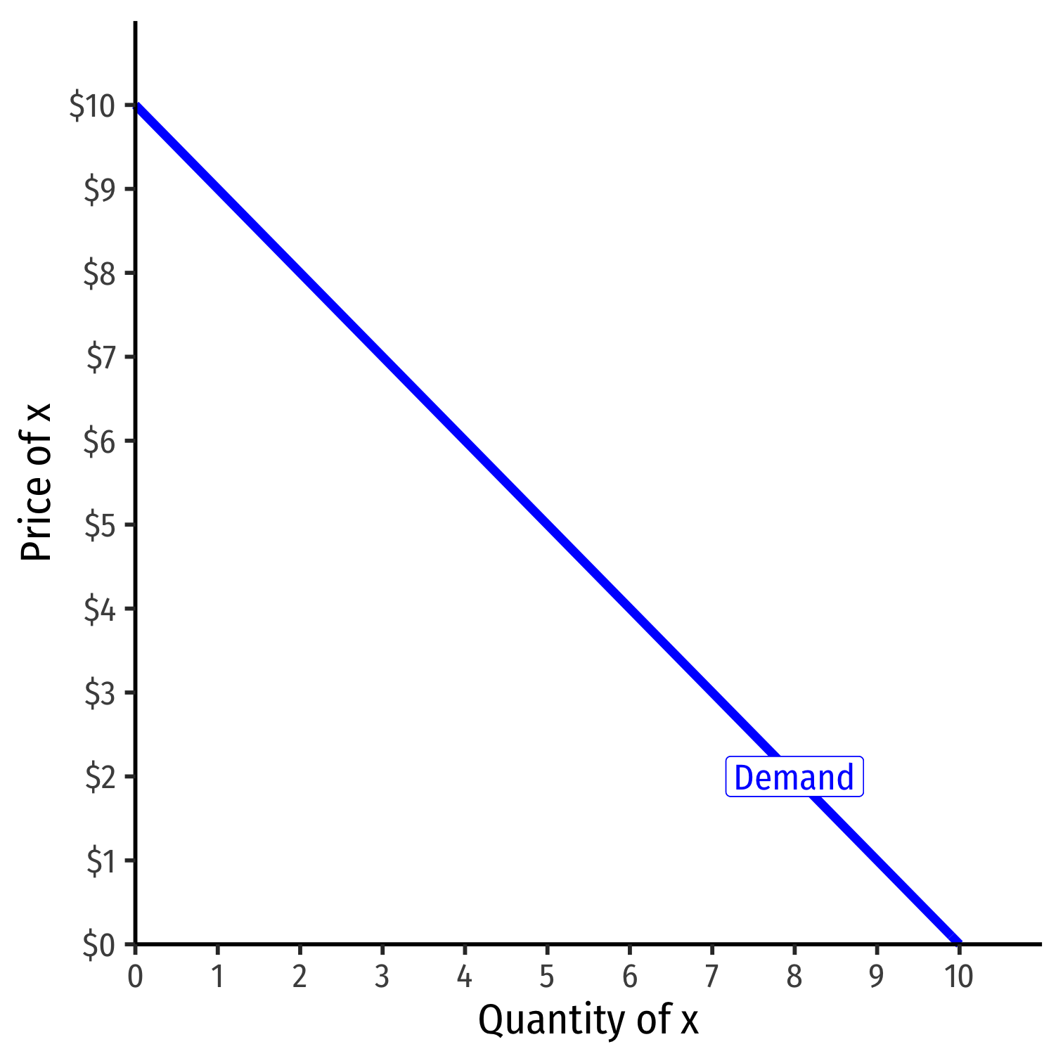
Inverse Demand Function
- Inverse demand function relates price to quantity
- Take demand function and solve for p
Example: p=10−q
- Vertical intercept ("Choke price"): price where qD=0 ($10), just high enough to discourage any purchases

Inverse Demand Function
Read two ways:
Horizontally: at any given price, how many units person wants to buy
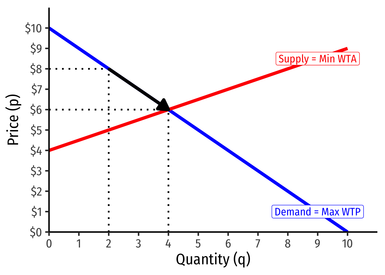
Vertically: at any given quantity, the maximum willingness to pay (WTP) for that quantity
- This way will be very useful later
Supply Function
- Supply function relates quantity to price
Example: q=2p−4
- Not graphable (wrong axes)!
Inverse Supply Function
- Inverse supply function relates price to quantity
- Take supply function, solve for p
Example: p=2+0.5q
- Graphable (price on vertical axis)!
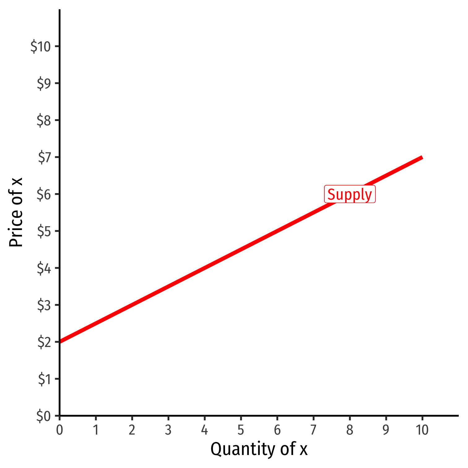
Inverse Supply Function
Example: p=2+0.5q
Slope: 0.5
Vertical intercept called the "Choke price": price where qS=0 ($2), just low enough to discourage any sales

Inverse Supply Function
Read two ways:
Horizontally: at any given price, how many units firm wants to sell
Vertically: at any given quantity, the minimum willingness to accept (WTA) for that quantity

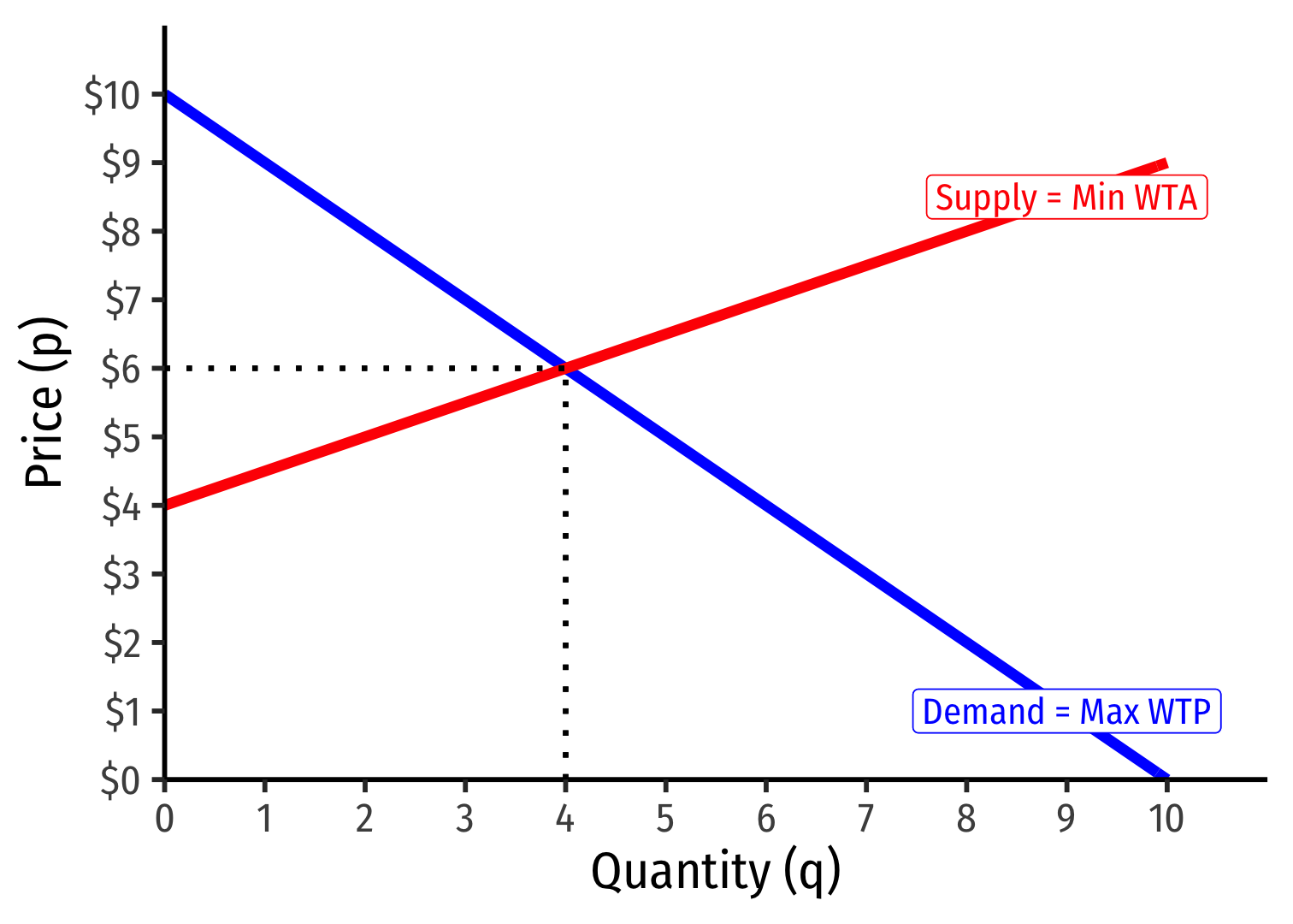
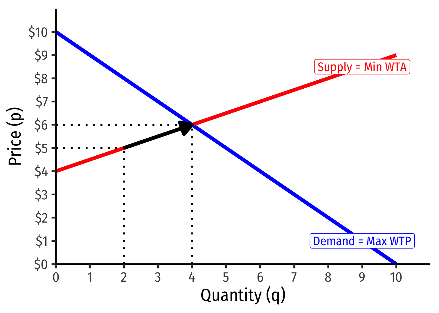
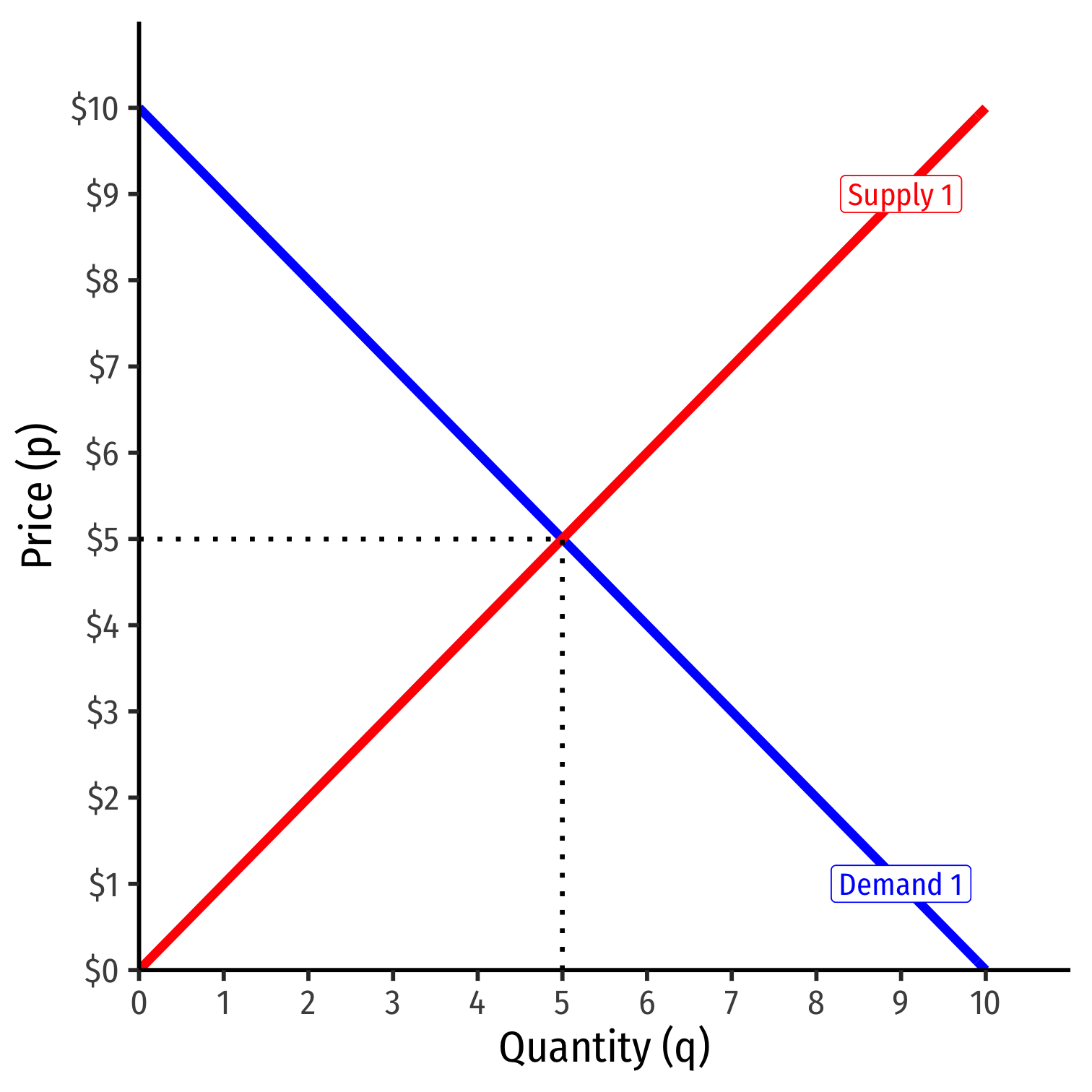
Market Equilibrium
Market-clearing (equilibrium) price (p∗): $6.00
Market-clearing (equilibrium) quantity exchanged (q∗): 4
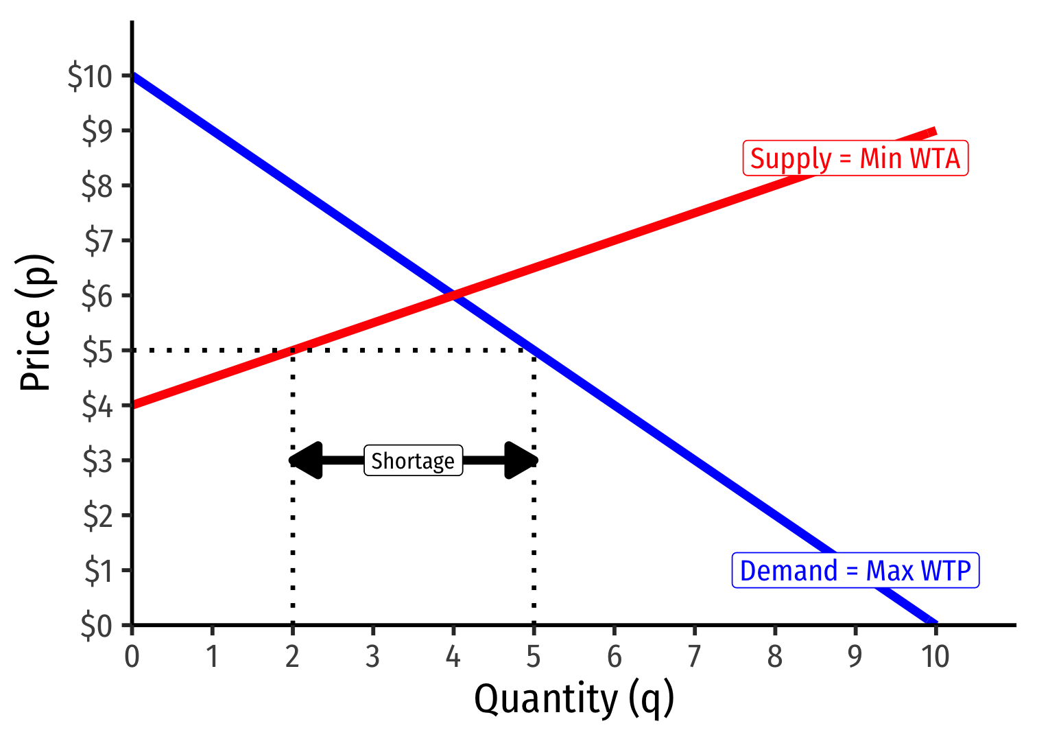
Excess Demand I
Example: Consider any price below $6, such as $5:
Qd=5Qs=2
Qd>Qs: excess demand
A shortage of 3 units
Excess Demand II
Example: Consider any price below $6, such as $5:
Qd=5Qs=2
Qd>Qs: excess demand
A shortage of 3 units
Sellers will not supply more than 2 units
For 2 units, some buyers are willing to pay more than $5
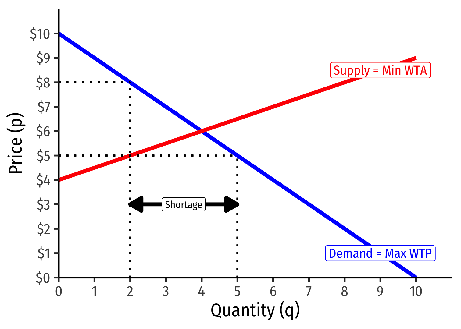
Excess Demand III
Example: Consider any price below $6, such as $5:
Qd=5Qs=2
Qd>Qs: excess demand
A shortage of 3 units
Buyers will raise their bids against one another, raising the price
At higher prices, sellers willing to sell more!
Until equilibrium, no pressure for change, Qd=Qs
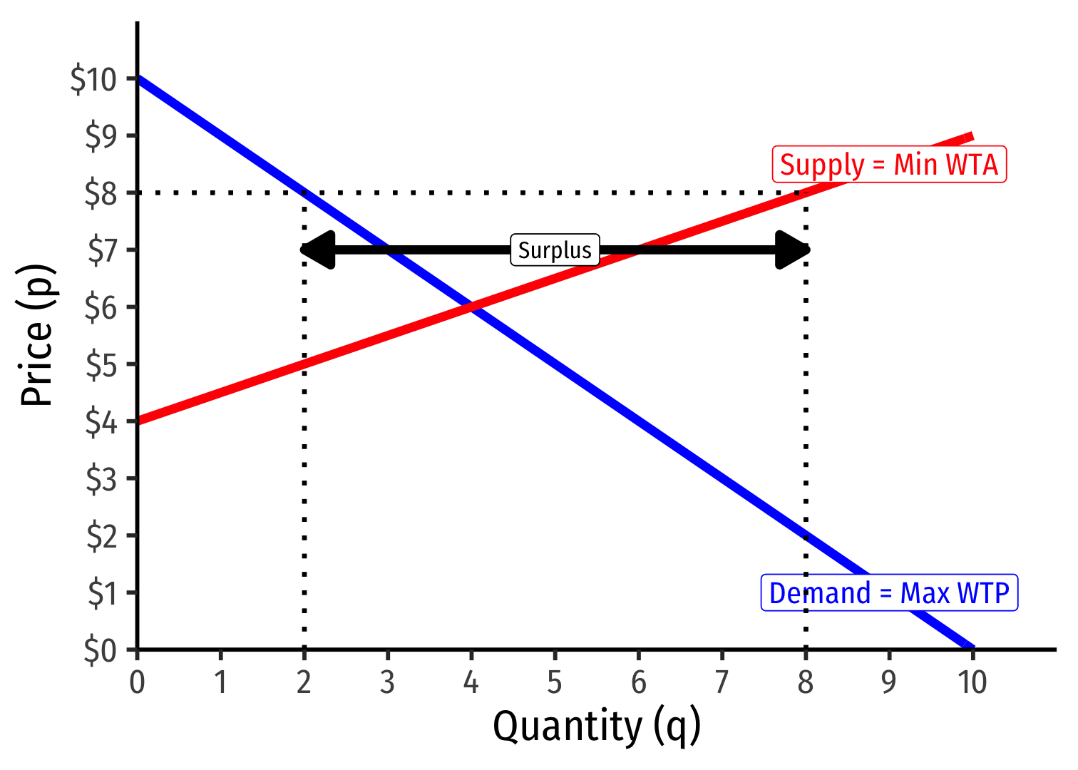
Excess Supply I
Example: Consider any price above $6, such as $7:
Qd=2Qs=8
Qd<Qs: excess supply
A surplus of 6 units
Excess Supply II
Example: Consider any price above $6, such as $7:
Qd=2Qs=8
Qd<Qs: excess supply
A surplus of 6 units
Buyers will not buy more than 2 units
For 2 units, some sellers willing to accept less than $8

Excess Supply III
Example: Consider any price above $6, such as $7:
Qd=2Qs=8
Qd<Qs: excess supply
A surplus of 6 units
Sellers will lower their asking prices against one another, lowering the price
At lower prices, buyers willing to buy more!
Until equilibrium, no pressure for change, Qd=Qs
Why Markets Tend to Equilibrate

Ceterus Paribus I
Supply function and demand function relate quantity (supplied or demanded) to price only
- Describes how buyers/sellers respond to changes in market price
Certainly there are many other factors that influence how much a buyer or seller will purchase at a particular price!
- income, preferences, prices of other goods, expectations, etc.
A supply or demand function (or graph) requires "ceterus paribus" (all else equal)

Recall (for example), Demand I
- A consumer's demand (for good x) depends on current prices & income:
qDx=qDx(m,px,py)
- How does demand for x change?
- Income effects (ΔqDxΔm): how qDx changes with changes in income
- Cross-price effects (ΔqDxΔpy): how qDx changes with changes in prices of other goods (e.g. y)
- (Own) Price effects (ΔqDxΔpx): how qDx changes with changes in price (of x)

See Class 1.7 for a reminder.
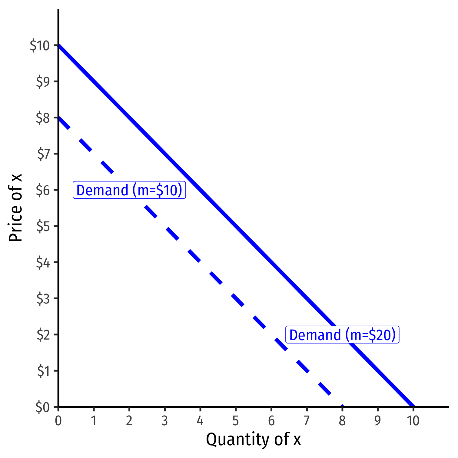
Recall (for example), Demand II
A change in one of the "determinants of demand" will shift demand curve!
- Change in income m
- Change in price of other goods py (substitutes or complements)
- Change in preferences or expectations about good x
- Change in number of buyers
Shows up in (inverse) demand function by a change in intercept (choke price)!
Again, see my Visualizing Demand Shifters
Ceterus Paribus II
Consider our demand function: qD=10−p
If the market price (p) changes (perhaps because supply changes), that results in a change in quantity demanded (qD)
- We move along the existing demand curve
Ceterus paribus has not been violated
Ceterus Paribus III
Consider our demand function: qD=10−p
If the something other than price changes (income, preferences, price of a complement, etc), that results in a change in demand
- We need to draw a new demand curve (or demand function)
qD=12−p
- Ceterus paribus has been violated
Ceterus Paribus IV
- There is a big difference between a change in "quantity demanded" and a change in "demand"!

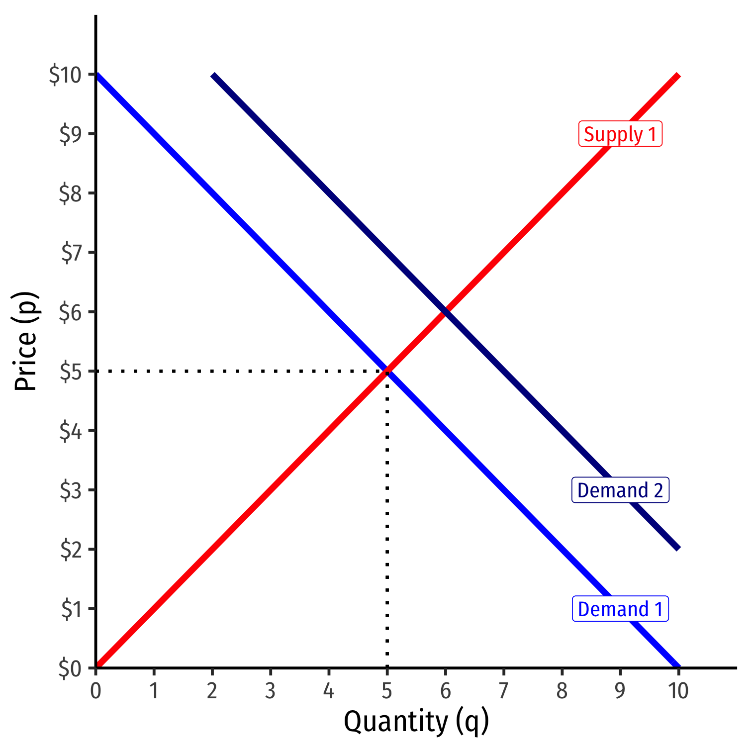
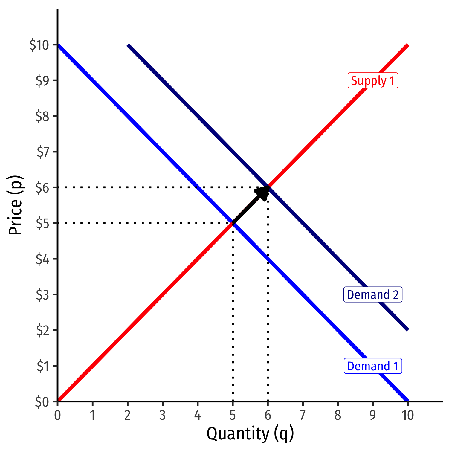
Increase in Demand

Increase in Demand
More individuals want to buy more of the good at every price
Entire demand curve shifts to the right
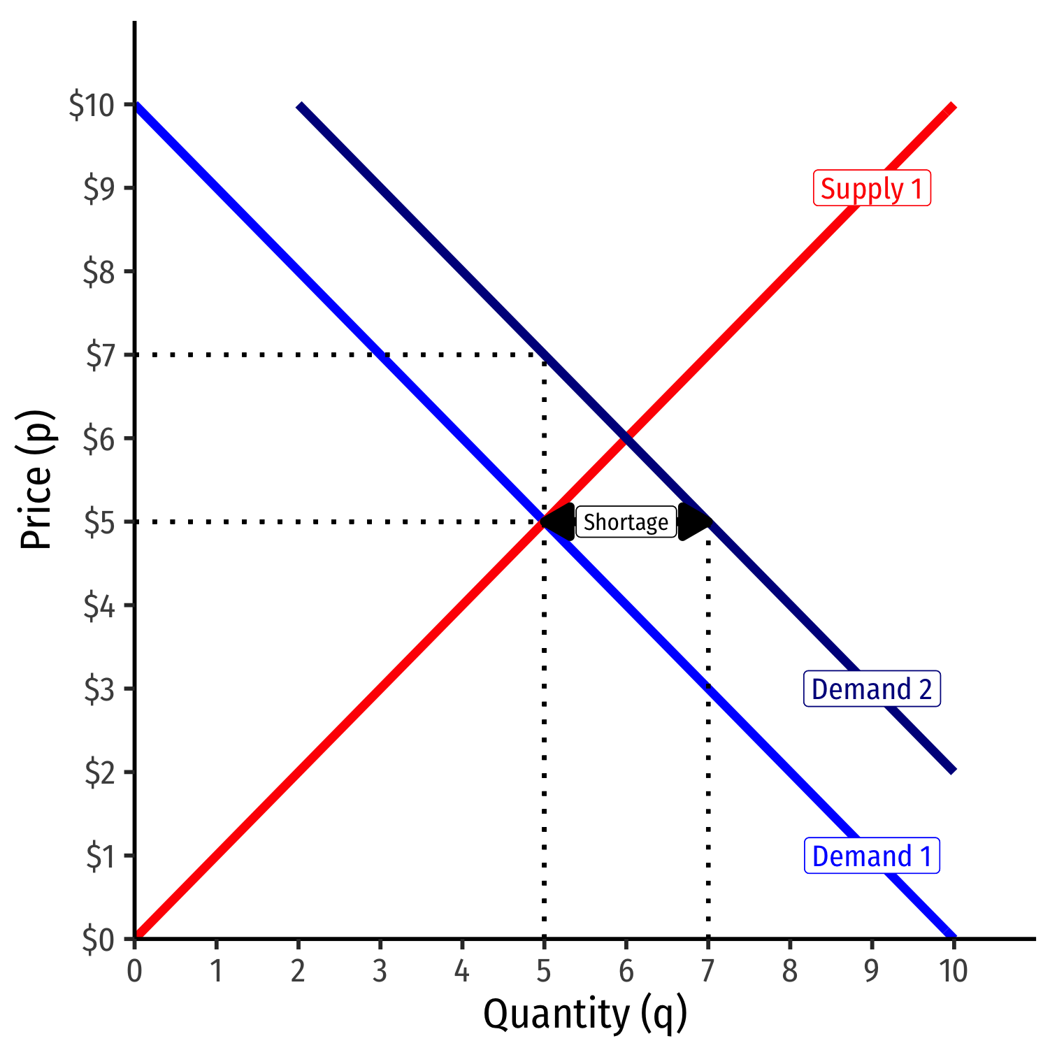
Increase in Demand
More individuals want to buy more of the good at every price
Entire demand curve shifts to the right
At the original market price, a shortage! (qD>qS)

Increase in Demand
More individuals want to buy more of the good at every price
Entire demand curve shifts to the right
At the original market price, a shortage! (qD>qS)
Some buyers willing to pay more at this quantity
Increase in Demand
More individuals want to buy more of the good at every price
Entire demand curve shifts to the right
At the original market price, a shortage! (qD>qS)
Some buyers willing to pay more at this quantity
Buyers raise bids, inducing sellers to sell more
Reach new equilibrium with:
- higher market-clearing price
- larger market-clearing quantity exchanged
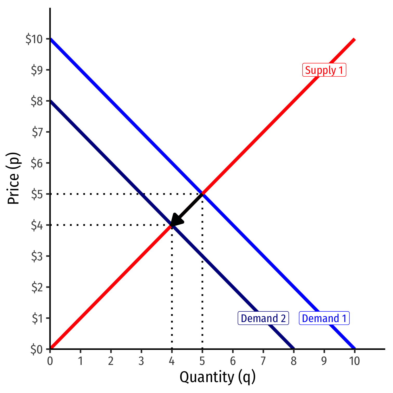
Decrease in Demand
Decrease in Demand
Fewer individuals want to buy less of the good at every price
Entire demand curve shifts to the left
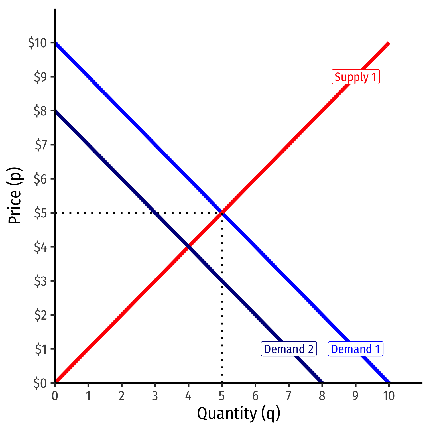
Decrease in Demand
Fewer individuals want to buy less of the good at every price
Entire demand curve shifts to the left
At the original market price, a surplus! (qD<qS)

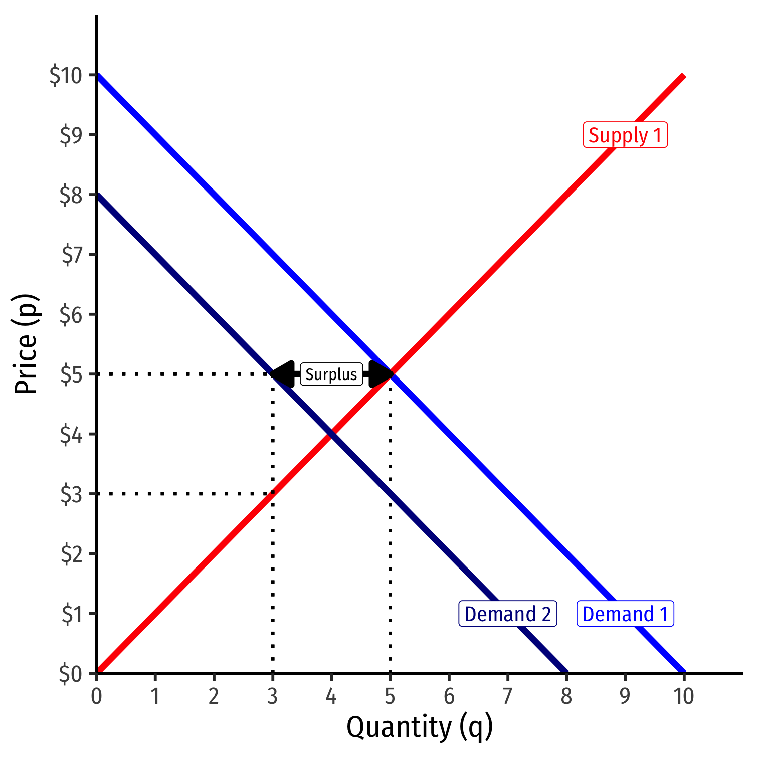
Decrease in Demand
Fewer individuals want to buy less of the good at every price
Entire demand curve shifts to the left
At the original market price, a surplus! (qD<qS)
Some sellers willing to accept less at this quantity
Decrease in Demand
Fewer individuals want to buy less of the good at every price
Entire demand curve shifts to the left
At the original market price, a surplus! (qD<qS)
Some sellers willing to accept less at this quantity
Sellers lower asks, inducing buyers to buy more
Reach new equilibrium with:
- lower market-clearing price
- smaller market-clearing quantity exchanged
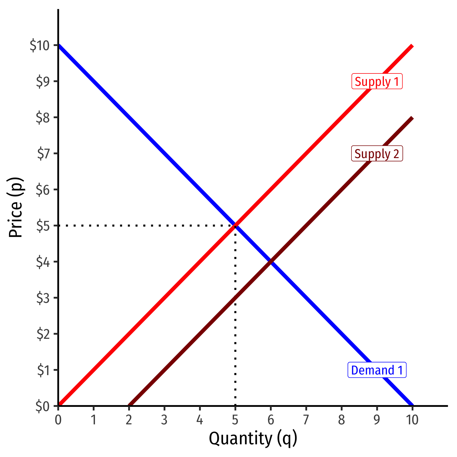
Increase in Supply

Increase in Supply
More individuals want to sell more of the good at every price
Entire supply curve shifts to the right
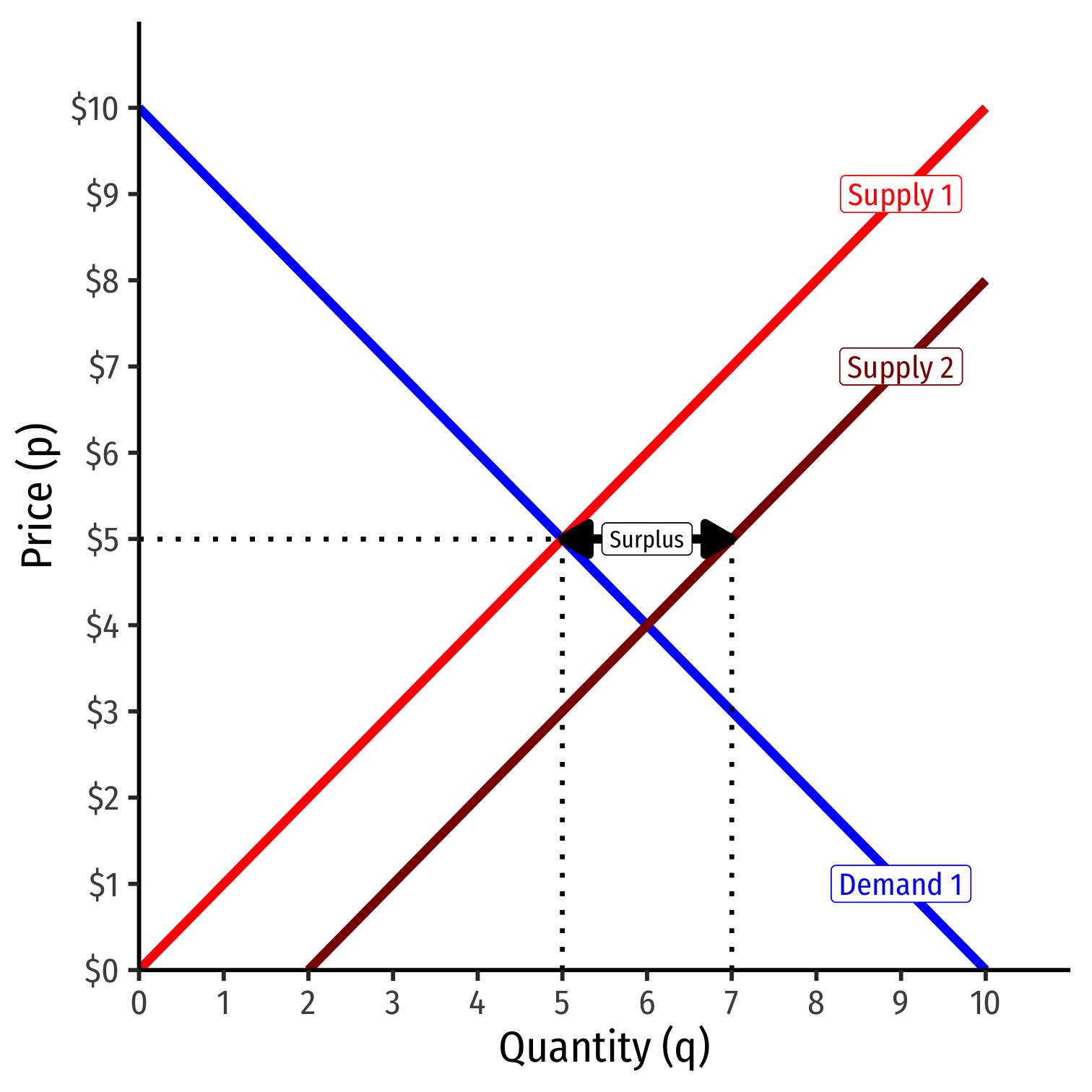
Increase in Supply
More individuals want to sell more of the good at every price
Entire supply curve shifts to the right
At the original market price, a surplus! (qD<qS)
Increase in Supply
More individuals want to sell more of the good at every price
Entire supply curve shifts to the right
At the original market price, a surplus! (qD<qS)
Some sellers willing to accept less at this quantity

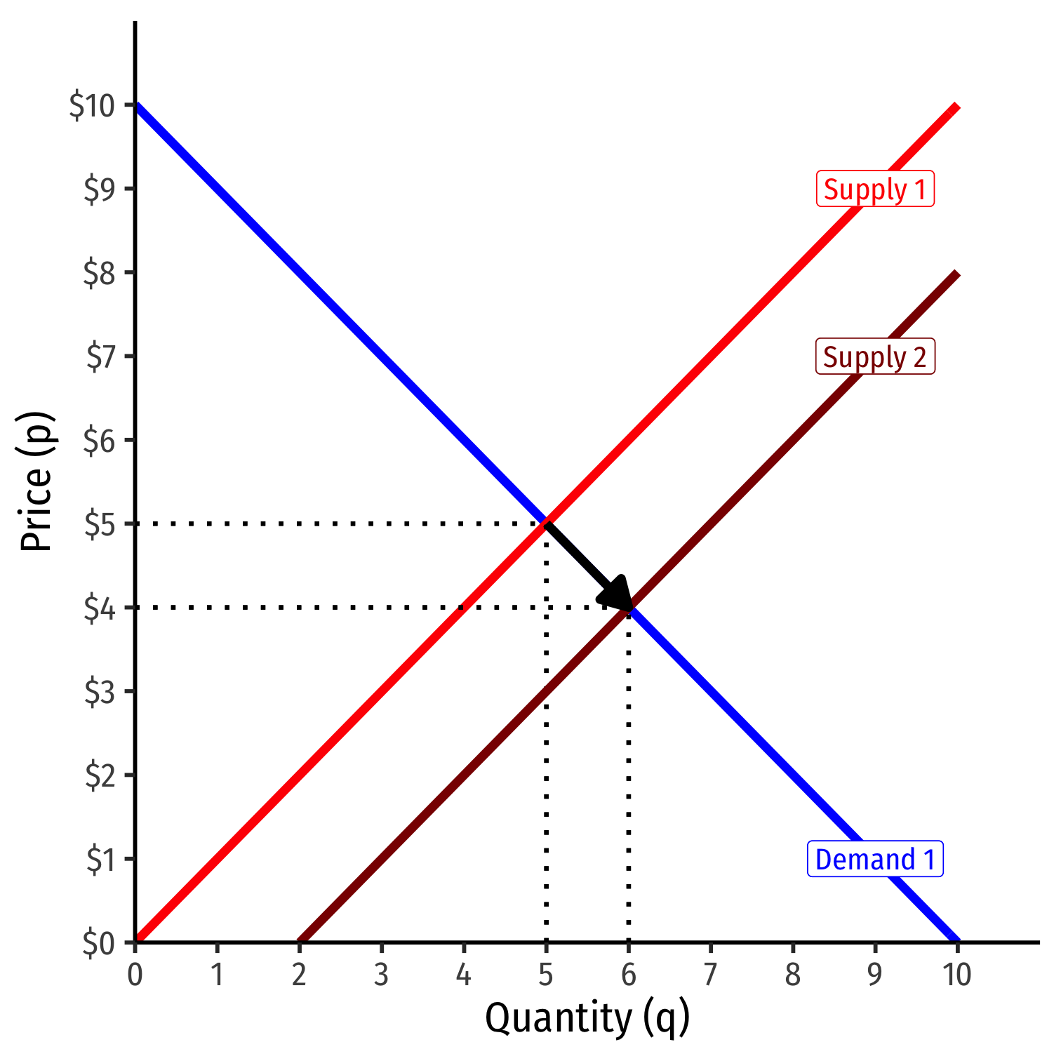
Increase in Supply
More individuals want to sell more of the good at every price
Entire supply curve shifts to the right
At the original market price, a surplus! (qD<qS)
Some sellers willing to accept less at this quantity
Sellers lower asks, inducing buyers to buy more
Reach new equilibrium with:
- lower market-clearing price
- larger market-clearing quantity exchanged
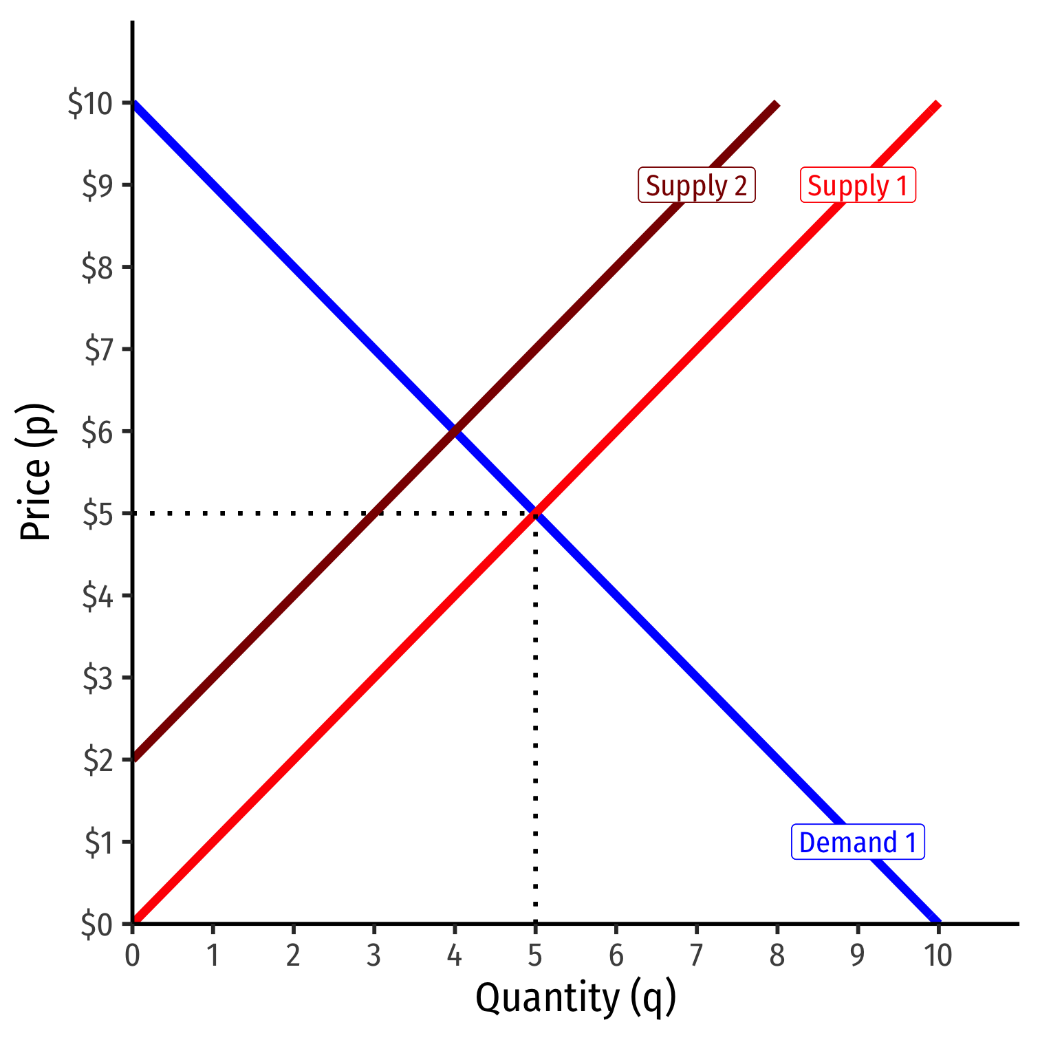
Decrease in Supply

Decrease in Supply
Fewer individuals want to sell less of the good at every price
Entire supply curve shifts to the left
Decrease in Supply
Fewer individuals want to sell less of the good at every price
Entire supply curve shifts to the left
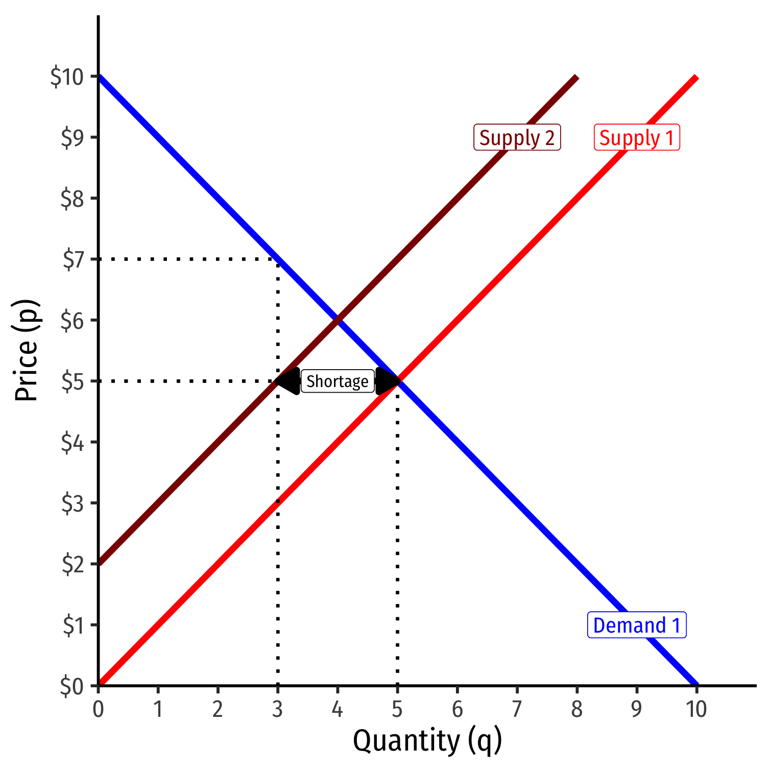
At the original market price, a shortage! (qD>qS)

Decrease in Supply
Fewer individuals want to sell less of the good at every price
Entire supply curve shifts to the left
At the original market price, a shortage! (qD>qS)
Some buyers willing to pay more at this quantity
Decrease in Supply
Fewer individuals want to sell less of the good at every price
Entire supply curve shifts to the left
At the original market price, a shortage! (qD>qS)
Some buyers willing to pay more at this quantity
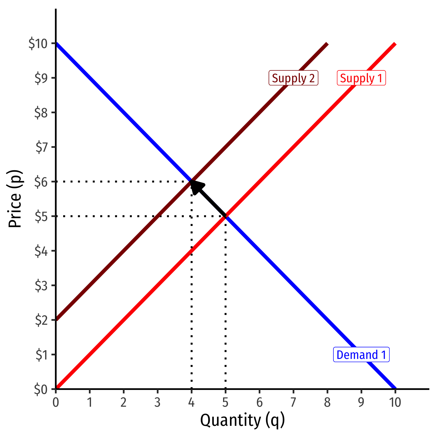
Buyers raise bids, inducing sellers to sell more
Reach new equilibrium with:
- higher market-clearing price
- smaller market-clearing quantity exchanged
Equilibrium Tendencies

Equilibrium is a tendency we can predict with our models
Buyers and sellers raise and lower their bids and asks to adjust to competition from other buyers and sellers, moving the market price
Ceterus paribus, market prices will settle on an equilibrium given existing conditions
But conditions are always changing (and so are prices)!