4.4 — Factor Markets
ECON 306 · Microeconomic Analysis · Fall 2020
Ryan Safner
Assistant Professor of Economics
safner@hood.edu
ryansafner/microF20
microF20.classes.ryansafner.com
Returning to Firms
Recall a firm uses technology that buys inputs, transforms them, and sells output q=f(k,l)
- We classified inputs into the factors of production: land, labor, capital
We assumed fixed factor prices
- show up in total cost =wL+rK
Where do they come from? Factor markets

Circular Flow

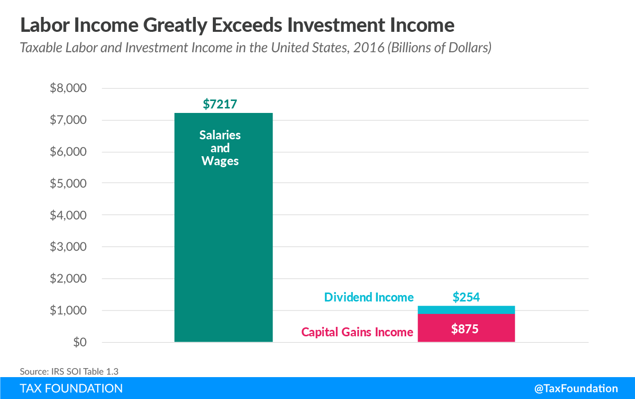
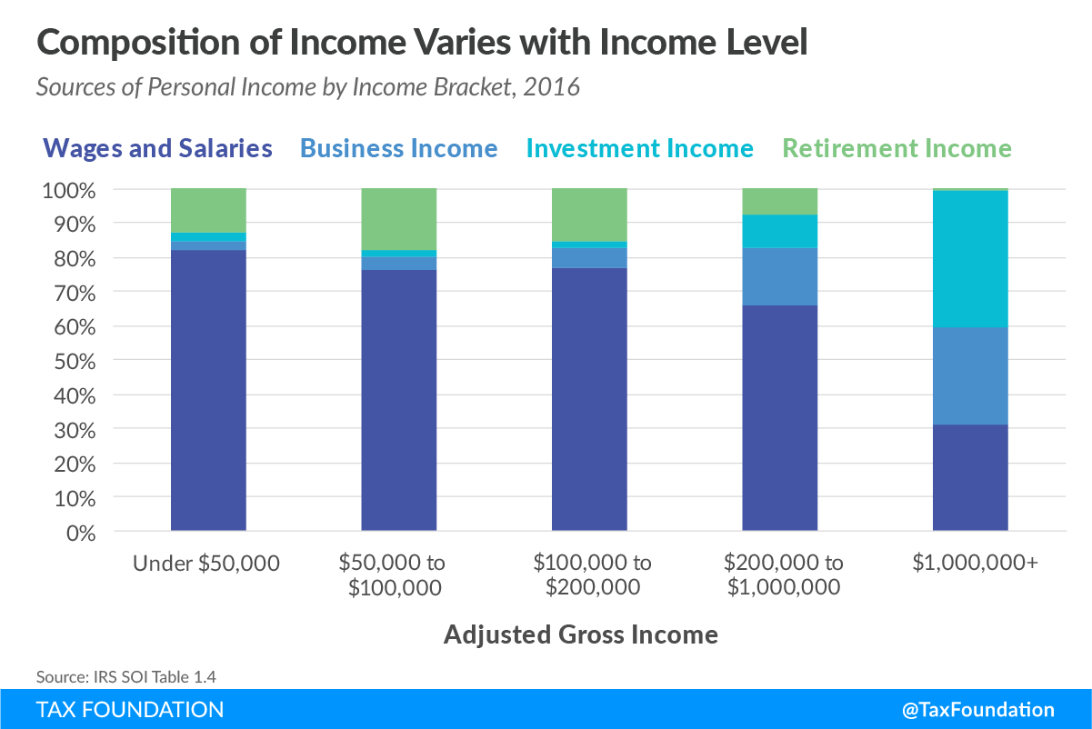
Firms’ Payments to Factors are Income To Households
| Income Type | Amount (2016) | Percent |
|---|---|---|
| Salaries and wages | $7217 Bn | 68.45% |
| Taxable pensions and annuities | $694 Bn | 6.58% |
| Partnership and S corporation net income | $629 Bn | 5.97% |
| Capital gains less losses | $621 Bn | 5.89% |
| Business net income | $389 Bn | 3.69% |
| Taxable Social Security benefits | $286 Bn | 2.71% |
| Taxable IRA distributions | $258 Bn | 2.45% |
| Ordinary dividends | $254 Bn | 2.41% |
| Total rental and royalty net income | $98 Bn | 0.93% |
| Taxable interest | $97 Bn | 0.92% |
Source: Tax Foundation, 2018
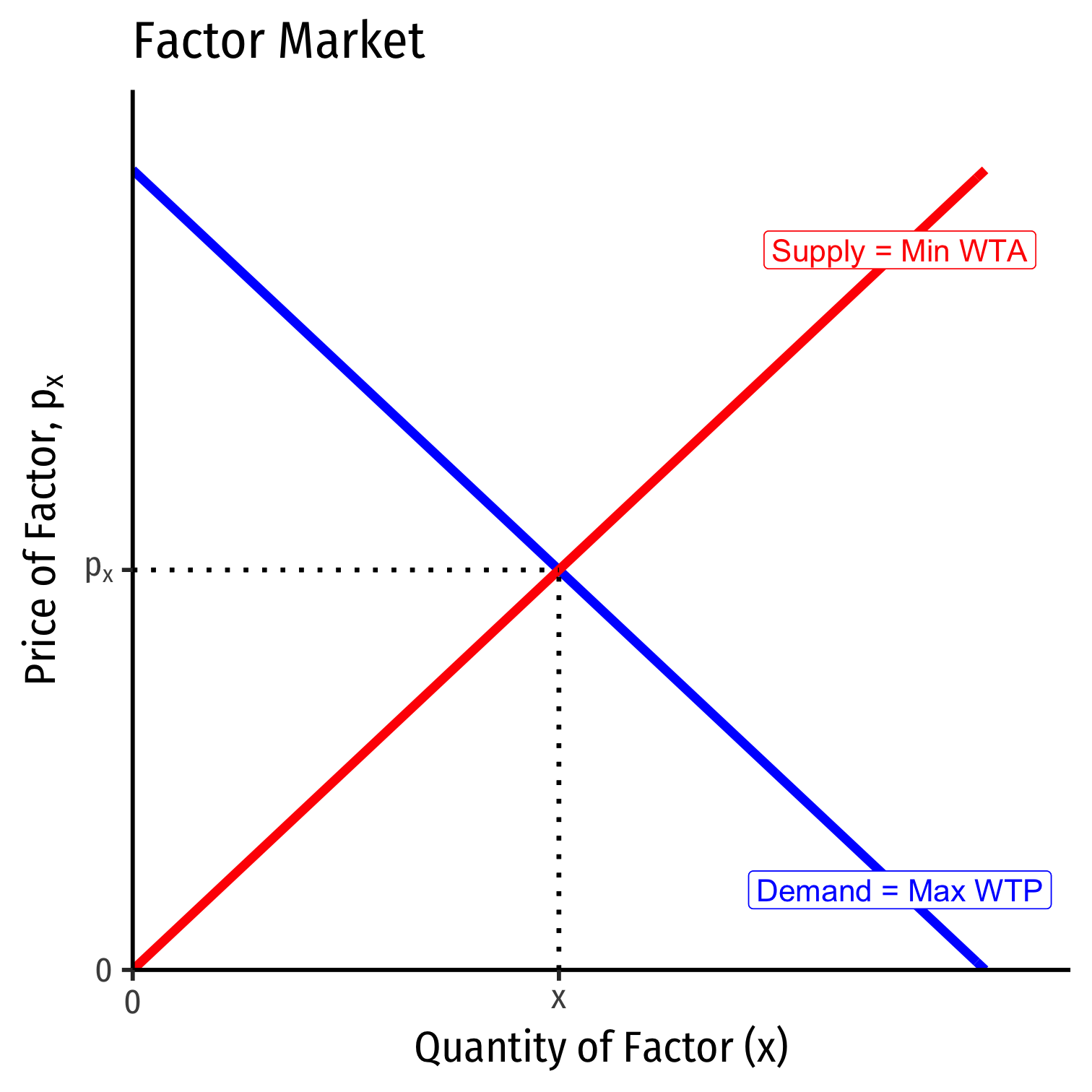
Supply and Demand in Factor Markets
The price of a factor is governed by the same market forces as output:
Supply of Factor: willingness of factor owners to accept and sell/rent their services to firms
- landowners, workers, capitalists, resource owners, suppliers
Demand for Factor: willingness of firms to pay for/hire factor services
Factor Market Prices and Opportunity Costs
- Factor price represents opportunity cost of hiring a factor for an alternative use
- Firms not only pay for direct use of a factor, but also indirectly for not using it in an alternate process!

Factor Market Prices and Opportunity Costs
- Example: a producer of hammers buys steel, pays (the opportunity cost) for "taking" the steel away from alternative uses

Factor Market Prices and Opportunity Costs
- Example: e.g. salary for a skilled worker must be high enough to keep them at their current firm, and not be attracted to other firms/industries

Example Factor Market: Labor Markets
Empirically, about 70% of total cost of production comes from labor
We’ll focus just on the market for labor as an example factor market
Can do the same for any factor market
- (e.g. capital, land, materials, etc.)

Labor Market for a Competitive Firm
Derived Demand in Factor Markets
Demand for factors is a "derived demand":
- Firm only demands inputs to the extent they contribute to producing sellable output
Firm faces a tradeoff when hiring more labor, as more labor ΔL creates:
- Marginal Benefit: Increases output and thus revenue
- Marginal Cost: Increases costs

Marginal Revenue Product (of Labor)
- Hiring more labor increases output (i.e. labor's MPL)
- Recall: MPL=ΔqΔL, where q is units of output
Marginal Revenue Product (of Labor)
Hiring more labor increases output (i.e. labor's MPL)
- Recall: MPL=ΔqΔL, where q is units of output
Additional output generates (i.e. labor's MR(q))
- Recall: MR(q)=ΔR(q)Δq, where R(q) is total revenue
Marginal Revenue Product (of Labor)
Hiring more labor increases output (i.e. labor's MPL)
- Recall: MPL=ΔqΔL, where q is units of output
Additional output generates (i.e. labor's MR(q))
- Recall: MR(q)=ΔR(q)Δq, where R(q) is total revenue
- Hiring more labor, on the margin, generates a benefit, called the marginal revenue product of labor, MRPL:
MRPL=MPL∗MR(q)
- i.e. the number of new products a new worker makes times the revenue earned by selling the new products
Marginal Revenue Product for Competitive Firms
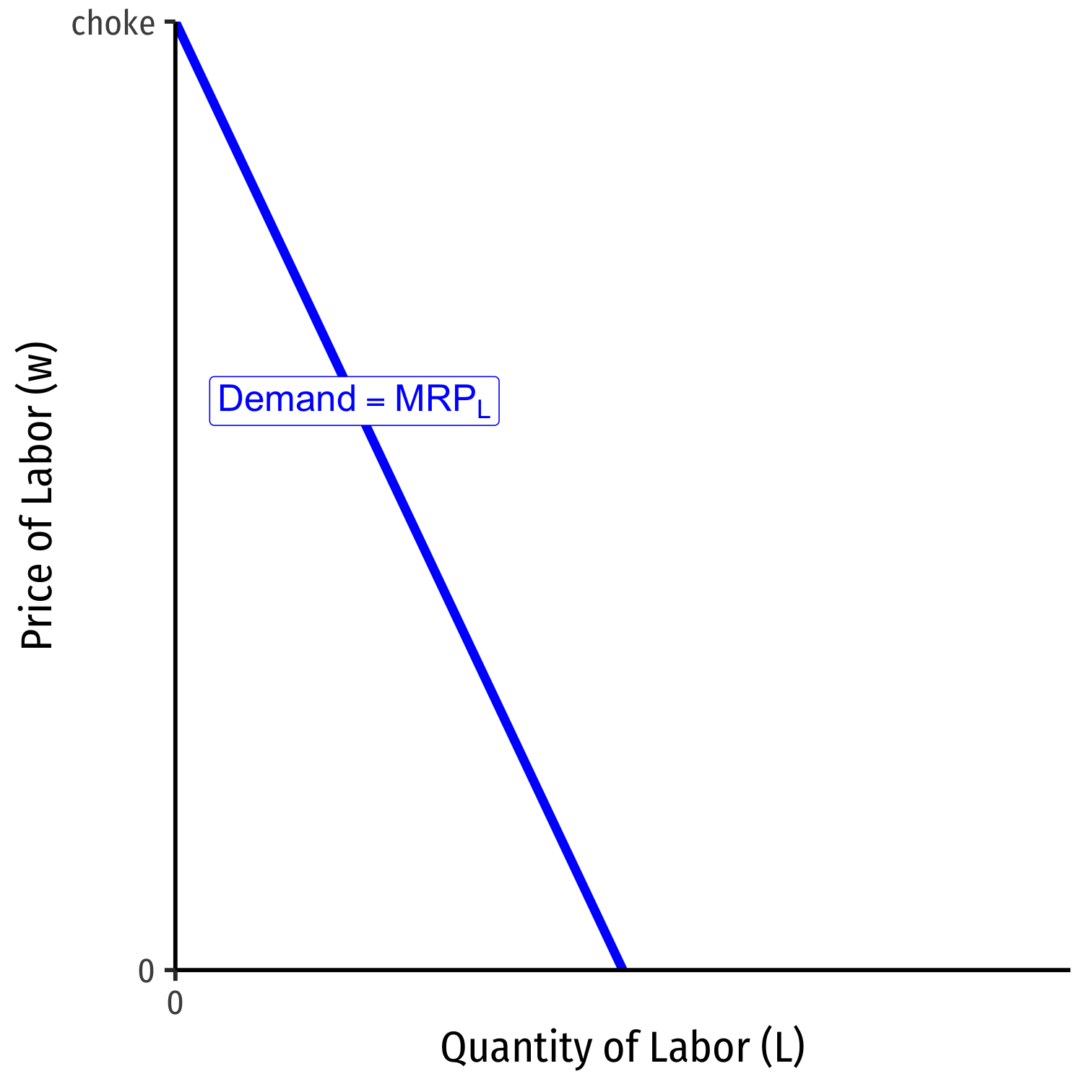
- This is the Firm's Demand for Labor:
MRPL=MPL∗MR(q)
- For a firm in a competitive (output) market, firm's MR(q)=p, hence:
MRPL=MPL∗p

Marginal Revenue Product for Competitive Firms
MRPL=MPL∗p
Marginal benefit of hiring labor, MRPL falls with more labor used
- production exhibits diminishing marginal returns to labor!
Choke price for labor demand: price too high for firm to purchase any labor
A Competitive Factor Market
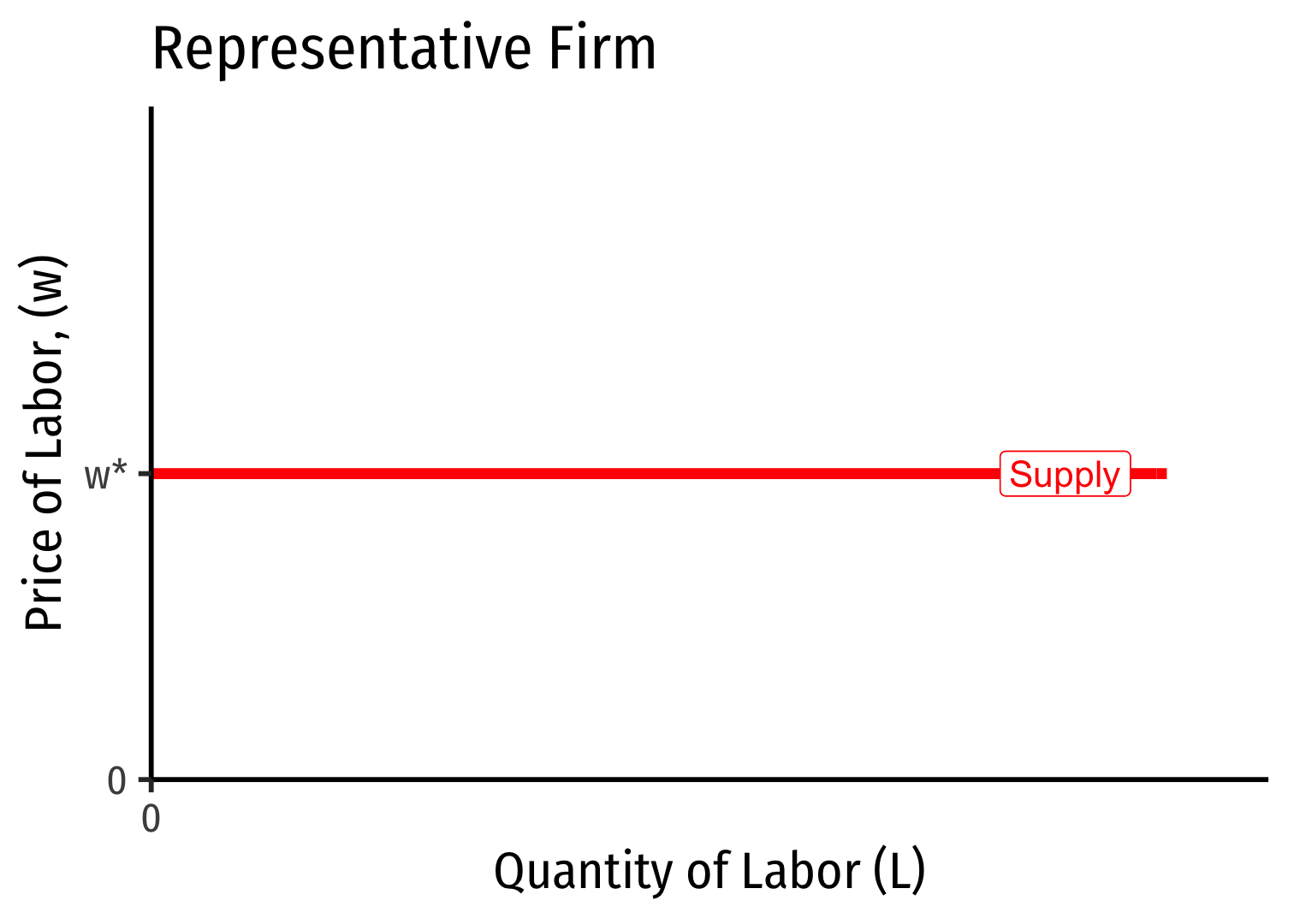
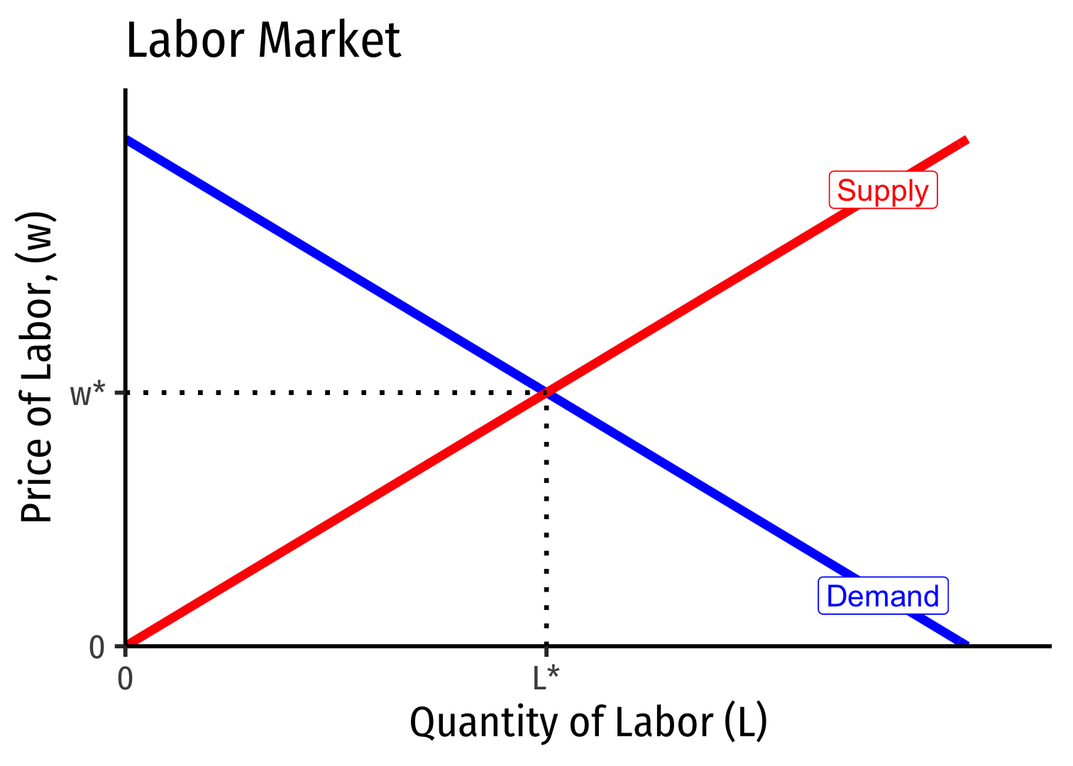
- If the factor market is competitive, labor supply for an individual firm is perfectly elastic at the market price of labor (w∗)
A Brief Digression on Economic Rents I
Recall market supply is the minimum willingness to accept, the minimum price necessary to bring a resource to market (its opportunity cost)
But all (equivalent) labor is paid the market wage, w∗ determined by market labor supply and labor demand

A Brief Digression on Economic Rents II
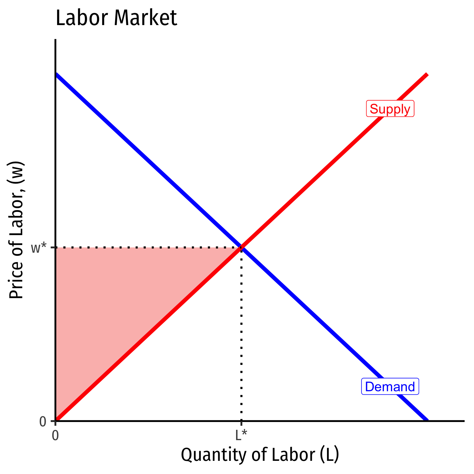
Some workers would have accepted a job for less than w∗
These inframarginal workers earn economic rent in excess of what is needed to bring them into the market (their opportunity cost)
A Brief Digression on Economic Rents III
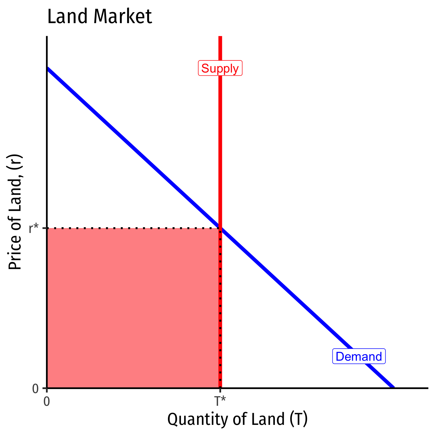
Consider a factor (such as land) for which the supply is perfectly inelastic (e.g. a fixed supply)
Then the entire value of the land is economic rent!
The less elastic the supply of a factor, the more economic rent it generates!
Labor Supply and Firm's Demand for Labor
We've seen a falling MRPL, the marginal benefit of hiring labor
Marginal cost of hiring labor, w, remains constant
- so long as firm is not a big purchaser (has no market power) in the labor market
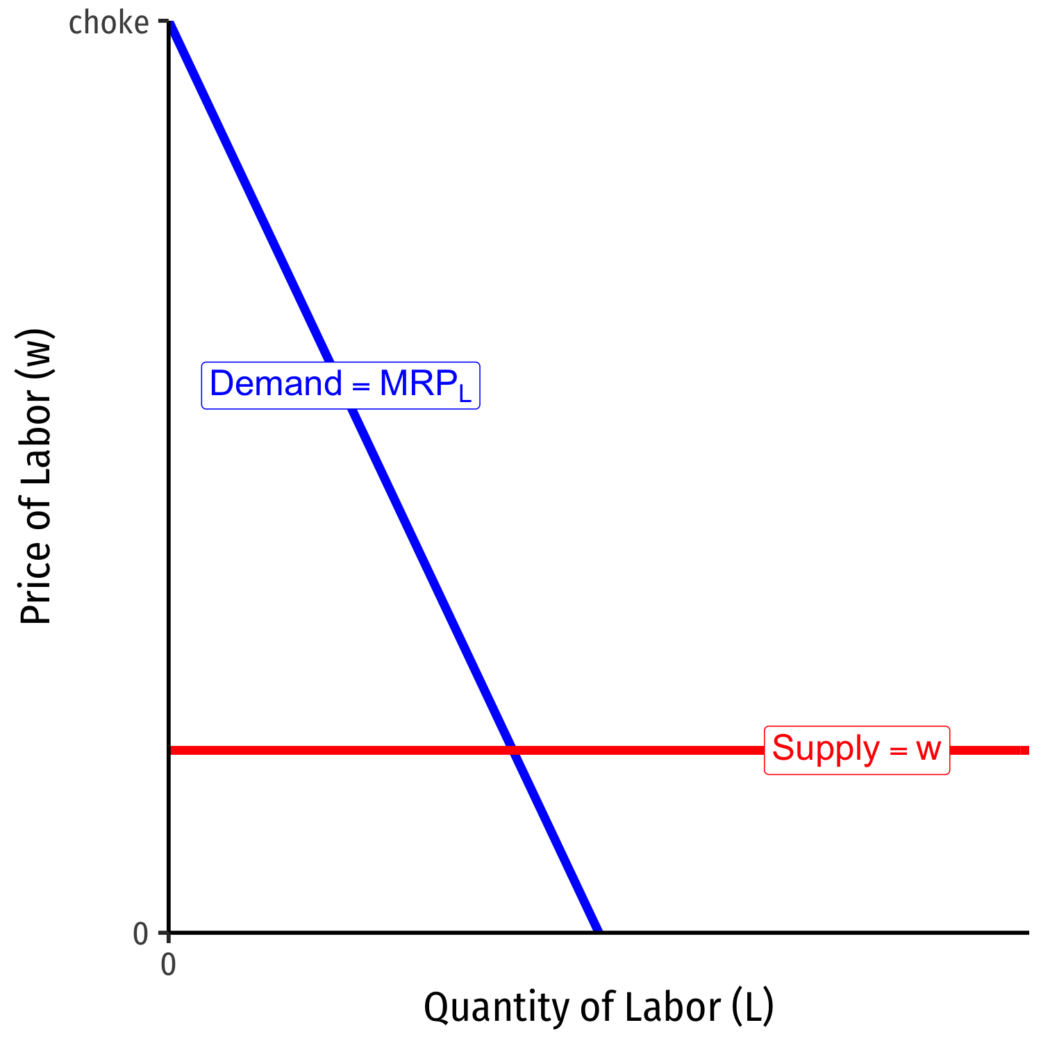
Labor Supply and Firm's Demand for Labor
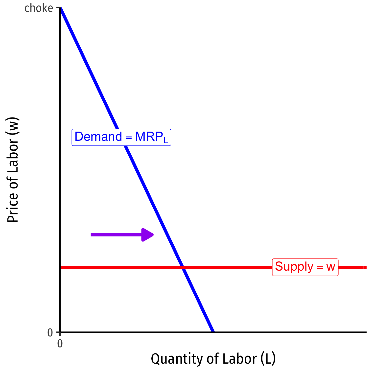
At low amounts of labor, marginal benefit MRPL>w marginal cost
Firm will hire more labor
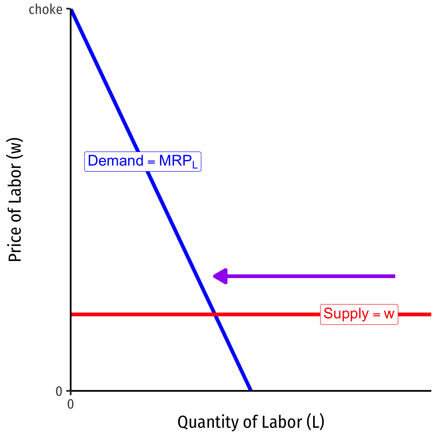
Labor Supply and Firm's Demand for Labor
At high amounts of labor, marginal benefit MRPL<w marginal cost
Firm will hire less labor
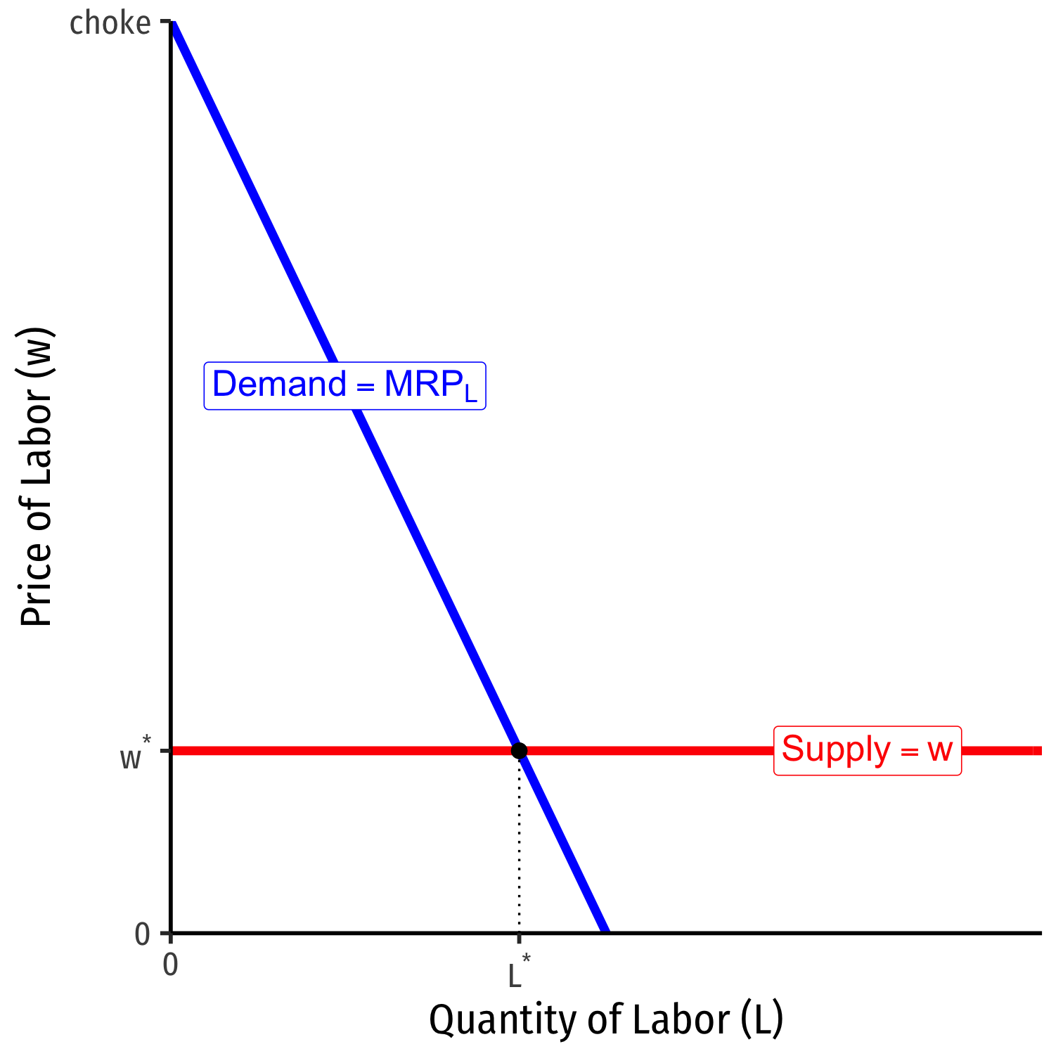
Labor Supply and Firm's Demand for Labor
Firm hires L∗ optimal amount of labor where w=MRPL
i.e. marginal cost of labor = marginal benefit of labor
Labor Supply and Firm's Demand for Labor
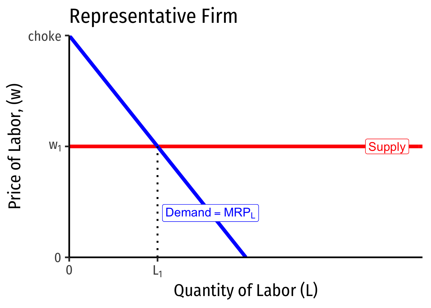
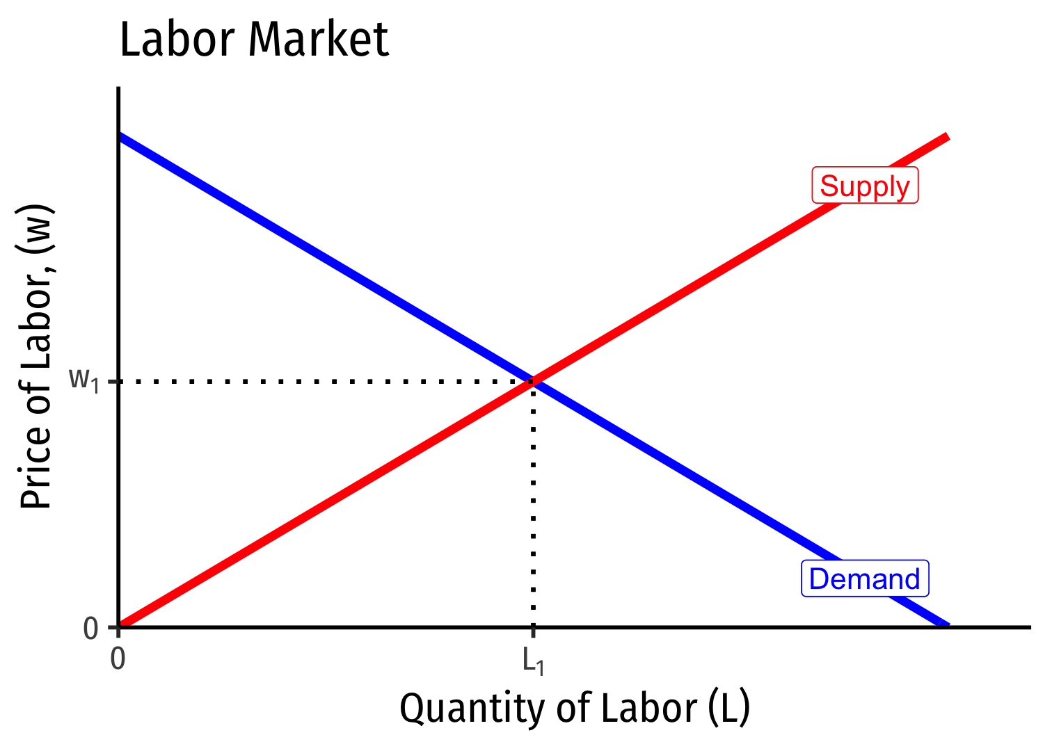
Labor Supply and Firm's Demand for Labor
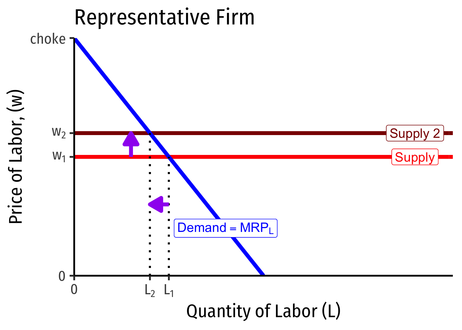
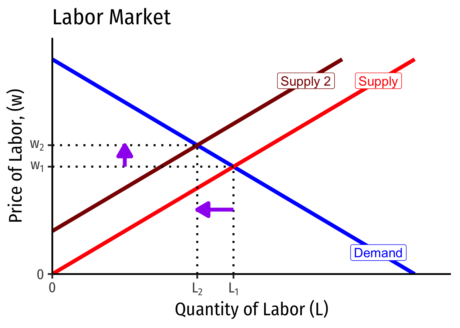
- If market supply of labor decreases, wages increase & firms hire fewer workers (and vice versa)
Example
Example: Victoria’s Tours is a travel company that offers guided tours of nearby mountain biking trails. Its marginal revenue product of labor is given by MRPL=1,000–40l, where l is the number of tour-guide weeks it hires and MRPL is measured in dollars per tour-guide week. The going market wage for Victoria’s Tours is $600 per tour-guide week.
What is the optimal amount of labor for Victoria’s Tours to hire?
At and above what market wage would Victoria’s Tours not want to hire anyone?
What is the most labor Victoria’s Tours would ever hire, given its marginal revenue product?
Labor Demand for a Monopoly
Labor Demand for Competitive vs. Monopolist Firm
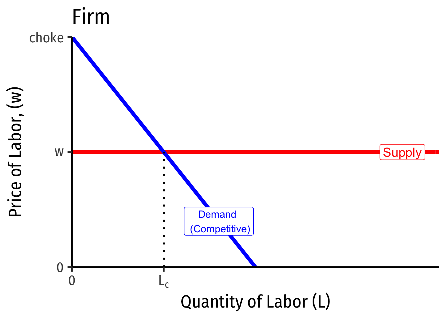
Recall a firm's demand for labor: MRPL=MPL∗MR(q)
A firm in a competitive output industry has its MR(q)=p
- So we saw its Labor Demand, MRPL=MPL∗p
Labor Demand for Competitive vs. Monopolist Firm

Recall if firm is a monopolist in its output industry, its MR(q)<p
- So its Labor Demand, MRPL=MRPL∗MR(q)
Since MR(q)<p, a monopoly in its output industry will always have lower demand for labor, and thus, hire less labor than a competitive firm
- Monopoly produces less output, so wants fewer inputs!
Labor Demand for Competitive vs. Monopolist Firm
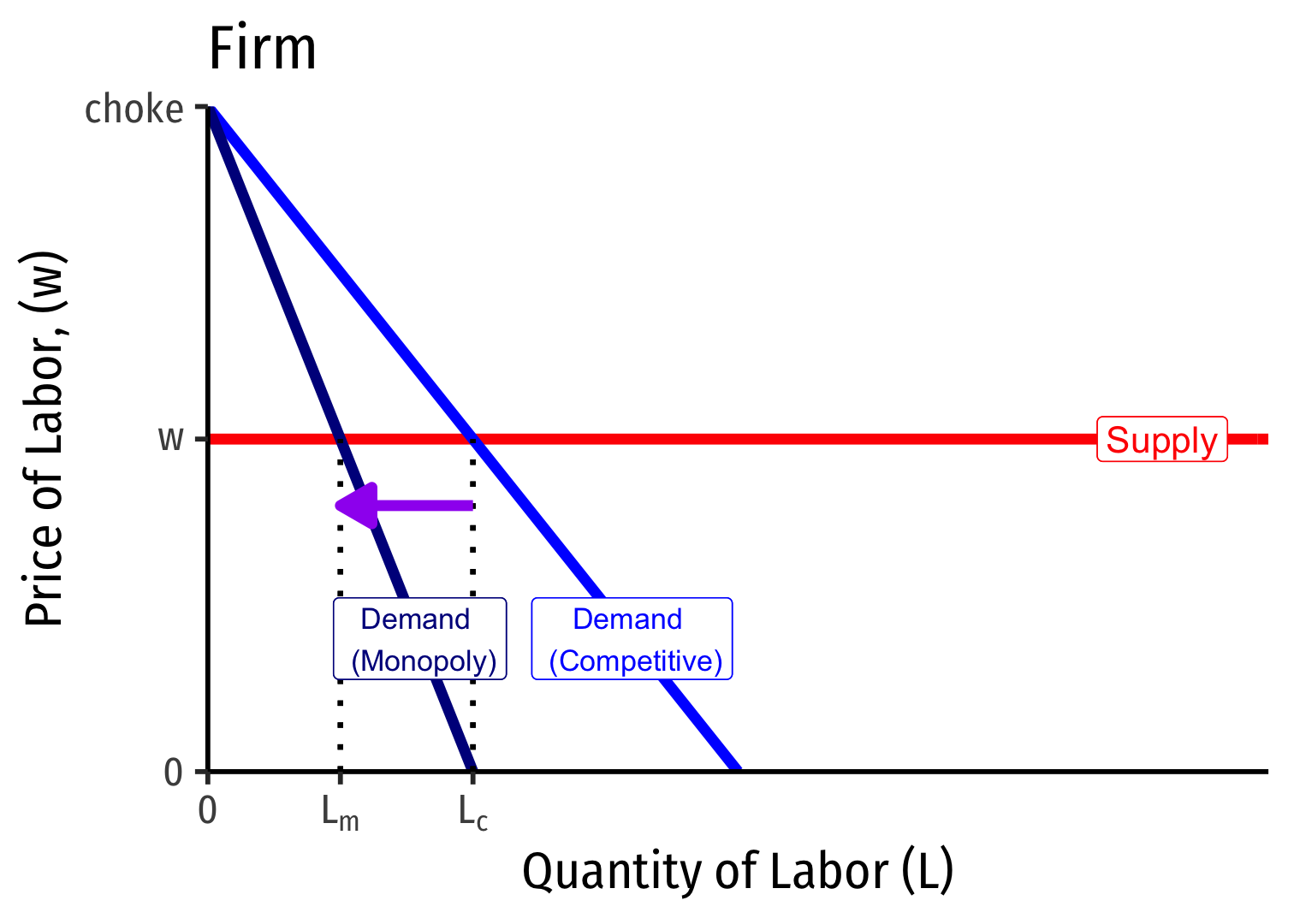
This is about the competitiveness of the output or "downstream" market
Here, both competitive firm and monopolist in downstream markets face the same perfectly elastic labor supply
- We've assumed no market power in the input or "upstream" market (for labor)
We next consider market power in the upstream (labor) market...
Monopsony Power
Monosony
What if the firm has market power in a factor market?
Consider extreme example: monopsony: a factor market with a single buyer

Monosony and Market Supply of Labor

Market power in hiring labor implies that the firm faces the whole market factor supply curve for labor
Market supply is upward sloping
Factor (inverse) supply describes minimum price workers are willing to accept to work
Monosony and Market Supply of Labor
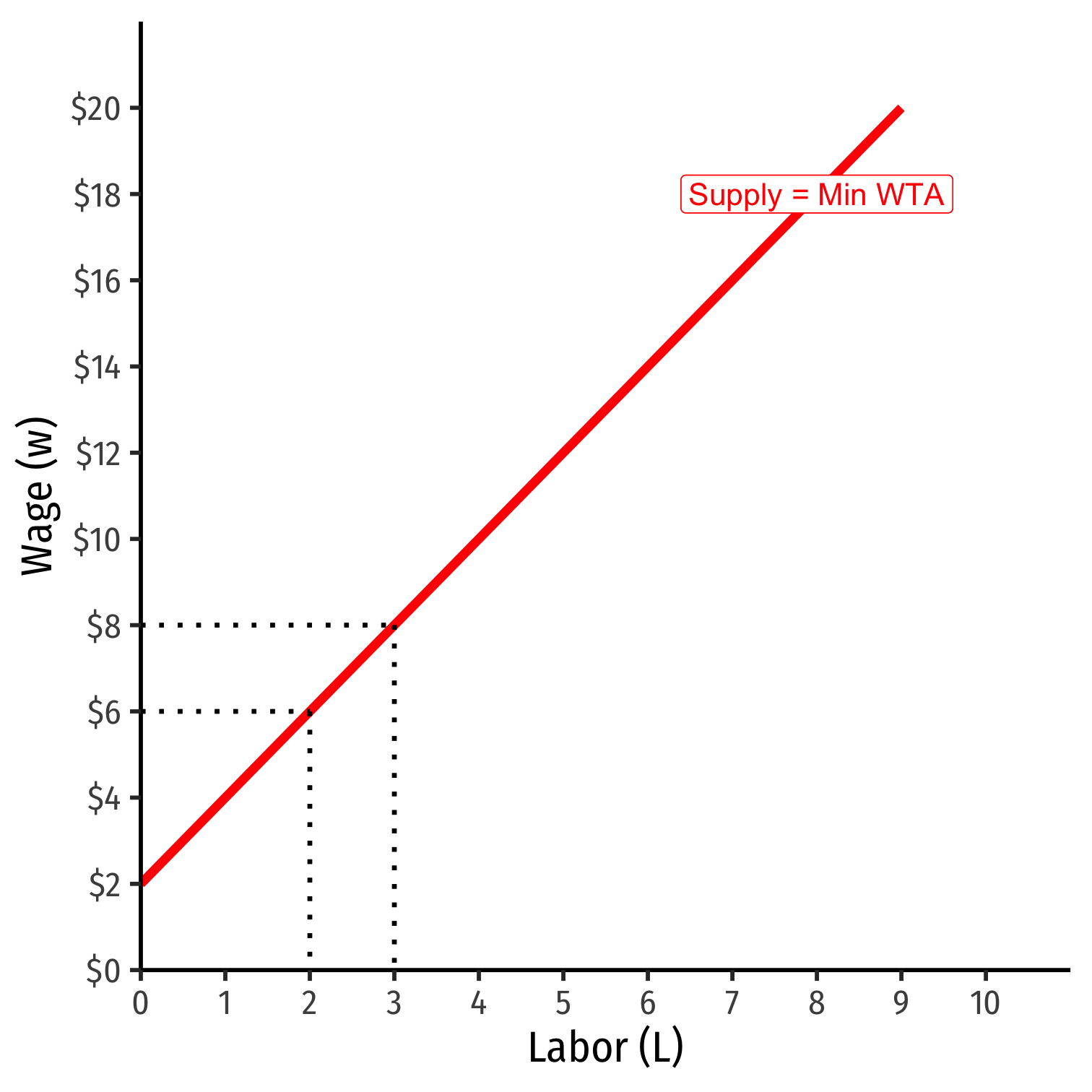
- As firm chooses to hire more L, must raise wages on all workers to hire them
Monosony and Market Supply of Labor
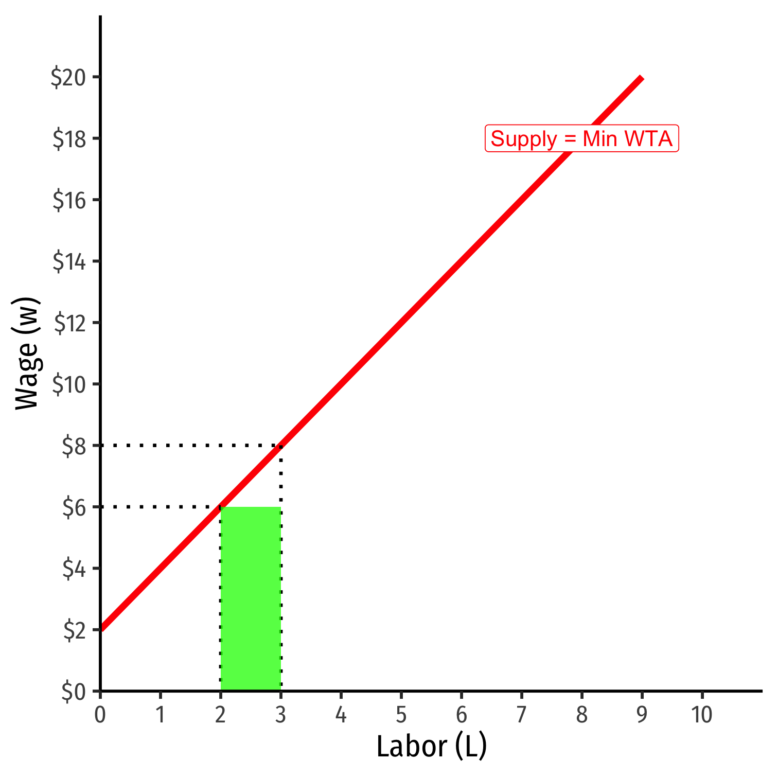
As firm chooses to hire more L, must raise wages on all workers to hire them
Output effect: increased cost from increased number of workers
Monosony and Market Supply of Labor
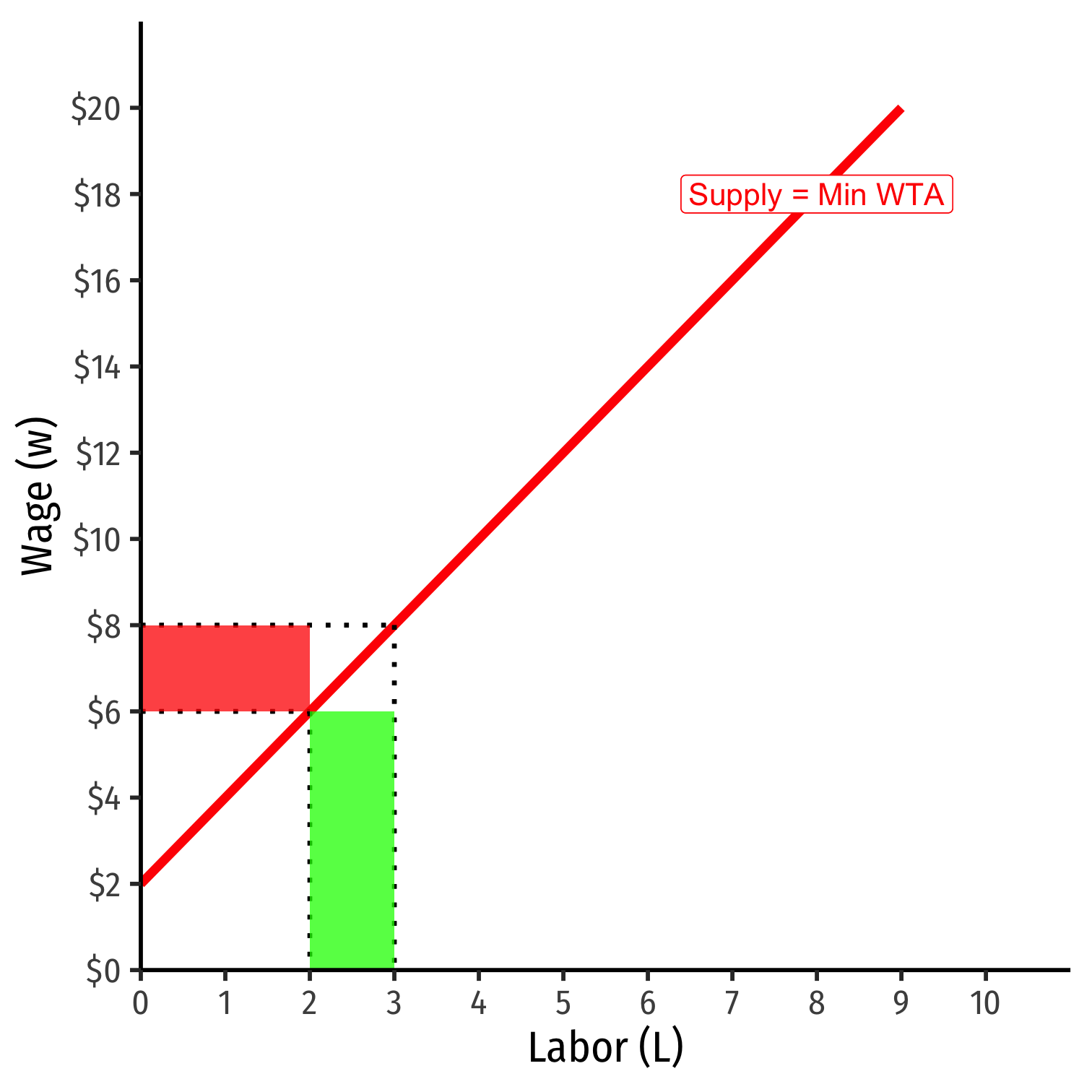
As firm chooses to hire more L, must raise wages on all workers to hire them
Output effect: increased cost from increased number of workers
Price effect: increased cost from raising wage for all workers
Monopsony and Marginal Cost of Labor I
- If monopsonist wants to hire more labor, ΔL, its labor cost C(L) would change by:
ΔC(L)=wΔL + LΔw
Monopsony and Marginal Cost of Labor I
- If monopsonist wants to hire more labor, ΔL, its labor cost C(L) would change by:
ΔC(L)=wΔL + LΔw
- Output effect: increases number of labor hired (ΔL) times wage w per worker
Monopsony and Marginal Cost of Labor I
- If monopsonist wants to hire more labor, ΔL, its labor cost C(L) would change by:
ΔC(L)=wΔL + LΔw
Output effect: increases number of labor hired (ΔL) times wage w per worker
Price effect: raises wage per worker (Δw) on all workers hired (L)
Monopsony and Marginal Cost of Labor I
- If monopsonist wants to hire more labor, ΔL, its labor cost C(L) would change by:
ΔC(L)=wΔL + LΔw
Output effect: increases number of labor hired (ΔL) times wage w per worker
Price effect: raises wage per worker (Δw) on all workers hired (L)
Divide both sides by ΔL to get Marginal Cost of Labor, MC(L):
ΔC(L)ΔL=MC(L)=w+ΔwΔLL
- Compare: supply for a price-taking firm is perfectly elastic: ΔwΔL=0, so we saw MC(L)=w!
Monopsony and Marginal Cost of Labor II
- If we have a linear inverse supply function for labor of the form
w=a+bL
- a is the choke price (intercept)
- b is the slope
Monopsony and Marginal Cost of Labor II
- If we have a linear inverse supply function for labor of the form
w=a+bL
- a is the choke price (intercept)
- b is the slope
- Marginal cost of labor again is defined as:
MC(L)=w+ΔwΔLL
Monopsony and Marginal Cost of Labor II
- If we have a linear inverse supply function for labor of the form
w=a+bL
- a is the choke price (intercept)
- b is the slope
- Marginal cost of labor again is defined as:
MC(L)=w+ΔwΔLL
- Recognize that ΔwΔL is the slope, b, (riserun)
Monopsony and Marginal Cost of Labor II
- If we have a linear inverse supply function for labor of the form
w=a+bL
- a is the choke price (intercept)
- b is the slope
- Marginal cost of labor again is defined as:
MC(L)=w+ΔwΔLL
- Recognize that ΔwΔL is the slope, b, (riserun)
MC(L)=w+(b)LMC(L)=(a+bL)+bLMC(L)=a+2bL
Monopsony and Marginal Cost of Labor IV
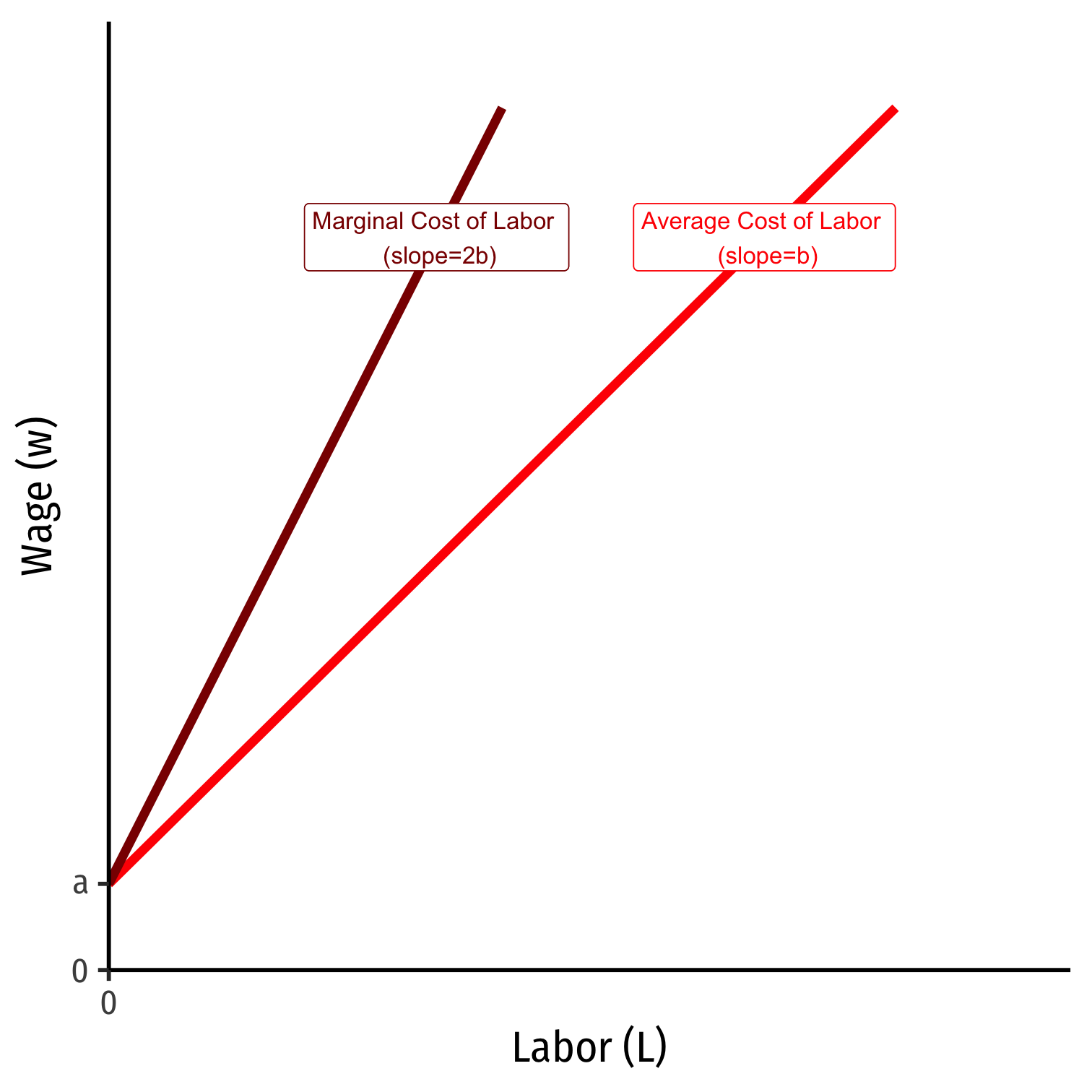
w(L)=a+bLMC(L)=a+2bL
- Marginal cost of labor starts at same intercept as Supply (average cost of labor) (a) with twice the slope (2b)
Note: If these past few slides have sounded familiar, this is the exact same process by which we derived a monopolist’s marginal revenue curve!
Monopsony's Hiring Decisions
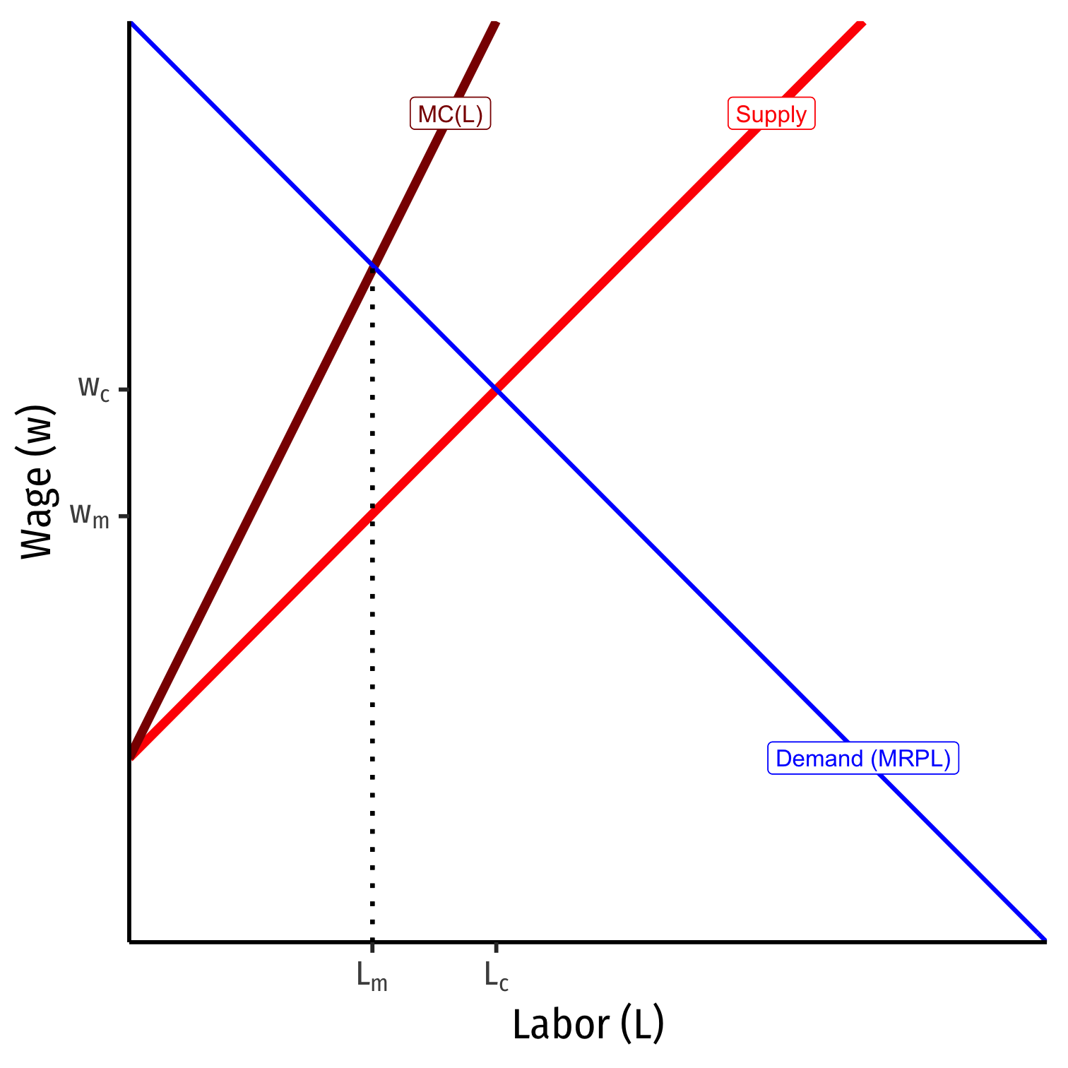
- Optimal quantity is where MC=MR
- Firm's MC(L)=MRPL
Monopsony's Hiring Decisions
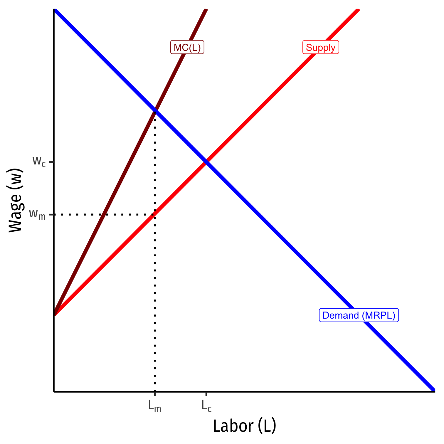
Optimal quantity is where MC=MR
- Firm's MC(L)=MRPL
Monopsonist faces entire market supply
- Can lower wages as low as workers’ minimum WTA (Supply)
Monopsonist’s Hiring Decisions
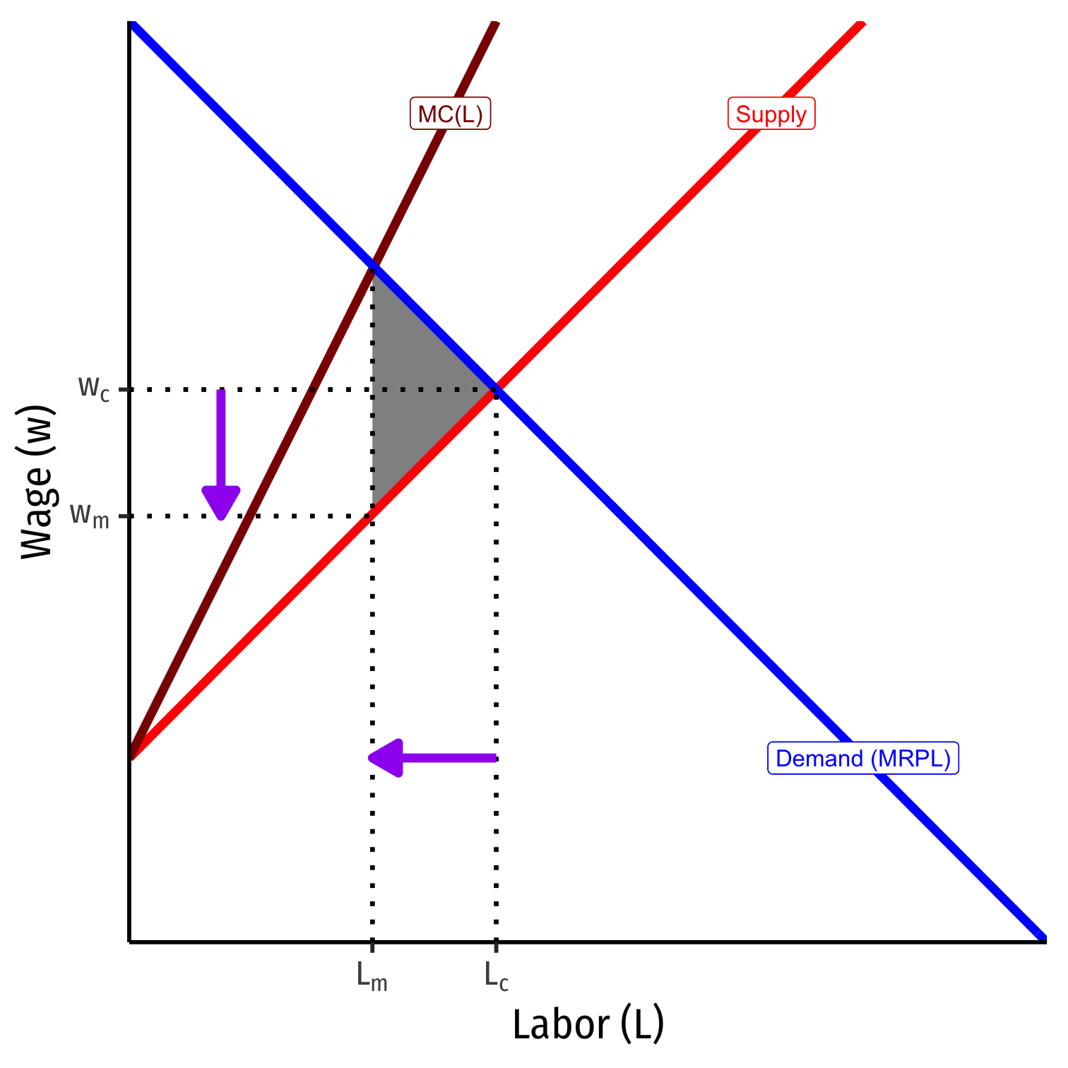
Optimal quantity is where MC=MR
- Firm's MC(L)=MRPL
Monopsonist faces entire market supply
- Can lower wages as low as workers' minimum WTA (Supply)
Compared to a competitive labor market (Lc,wc), monopsonist hires fewer workers and pays them lower wages (Lm,wm)
- Creates deadweight loss
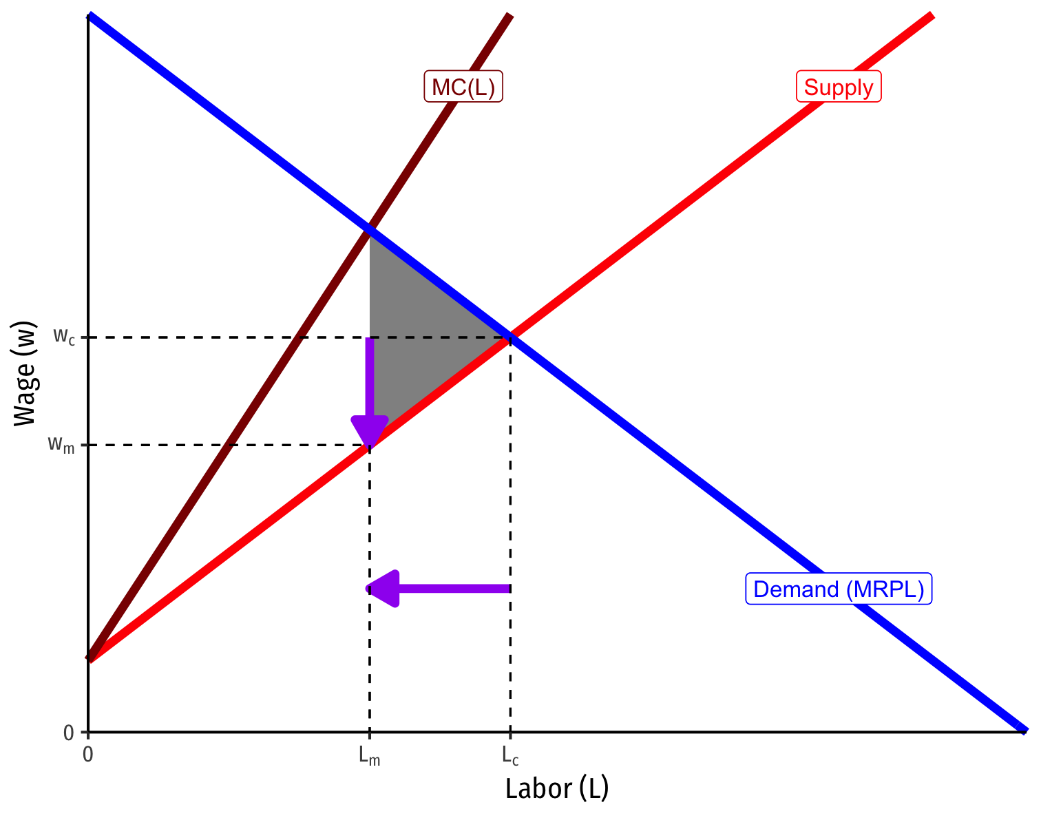
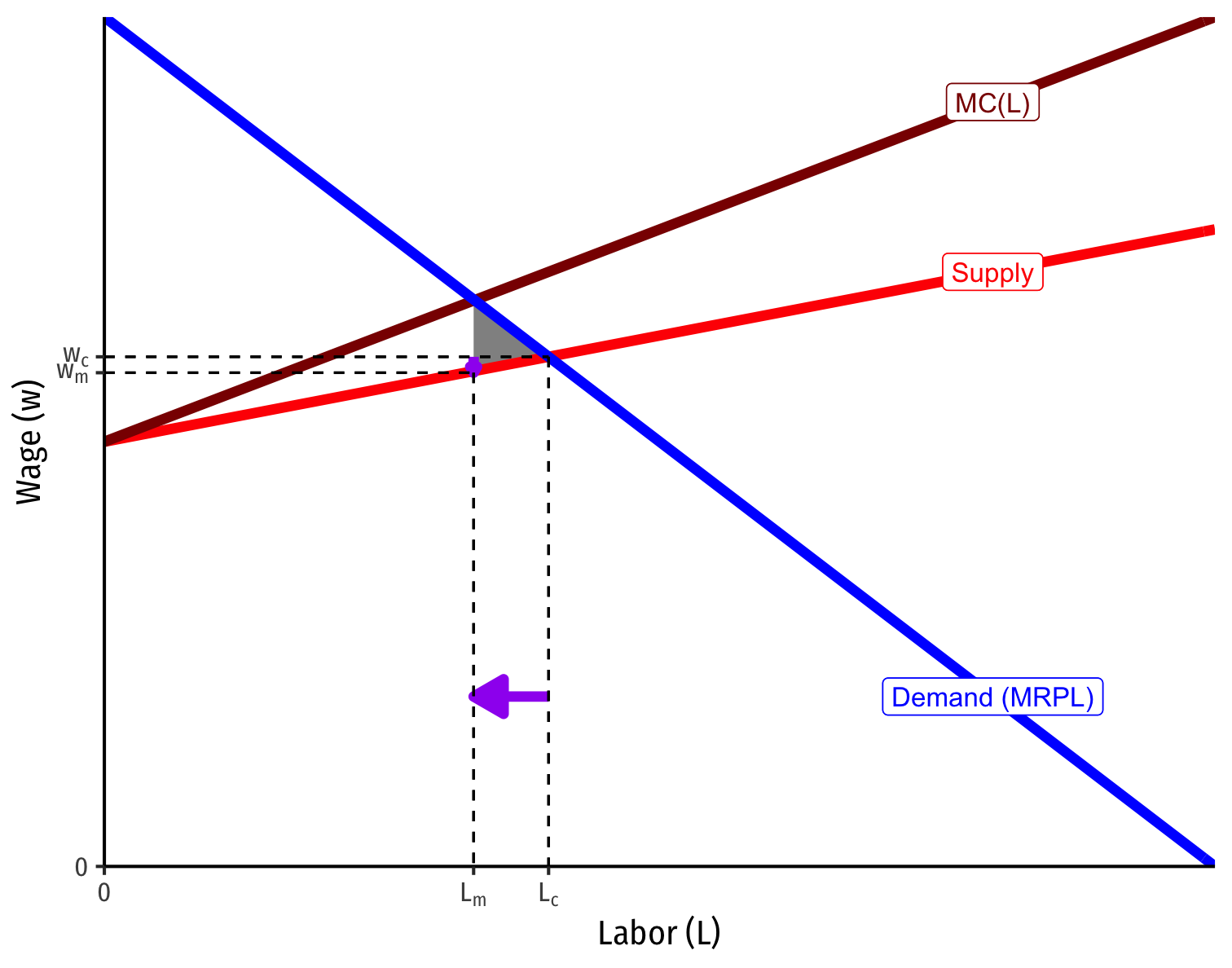
Monopsony Depends on Price Elasticity of Supply
The more (less) elastic labor supply, the less (more) monopsony power
Less Elastic Labor Supply Curve
More Elastic Labor Supply Curve
Monopoly Power in Labor Markets: Unions
Monopoly Power in Labor Markets: Unions
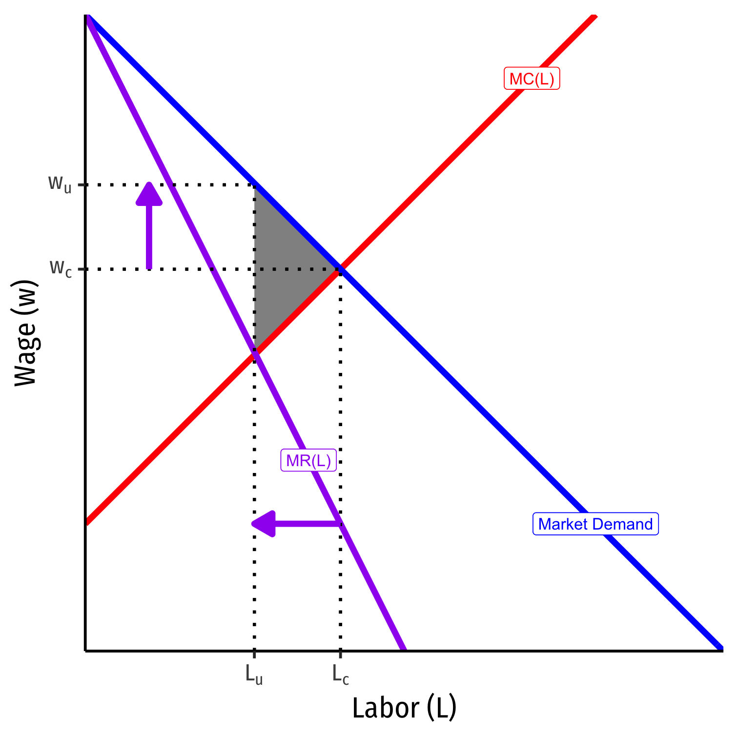
If seller/s of labor (workers) has market power, can act like a monopolist on the labor market
Example: A labor union
Faces entire market demand for labor, and thus its marginal revenue curve too
Acts like a monopolist, restricts Lu<Lc to push up wu>wc
The Problem of Bilateral Monopoly
What if both sides of the market have market power?
- A downstream monopsonist buyer vs. an upstream monopolist seller
This is the problem of bilateral monopoly
Find out more in my industrial organization course
- One solution is vertical integration: merge into a single firm across both markets

