2.4 — Costs of Production — Class Notes

Contents

Wednesday, September 23, 2020

Overview

Today we cover costs before we put them together next class with revenues to solve the firm’s (first stage) profit maximization problem. While it seems we are adding quite a bit, and learning some new math problems with calculating costs, we will practice it more next class, when put together with revenues.

Slides

• View Lecture Slides
• Download as PDF

Appendix

The Relationship Between Returns to Scale and Costs

There is a direct relationship between a technology’s returns to scaleIncreasing, decreasing, or constant

and its cost structure: the rate at which its total costs increaseAt a decreasing rate, at an increasing rate, or at a constant rate, respectively

and its marginal costs changeDecreasing, increasing, or constant, respectively

. This is easiest to see for a single input, such as our assumptions of the short run (where firms can change l but not ˉk):

q=f(ˉk,l)

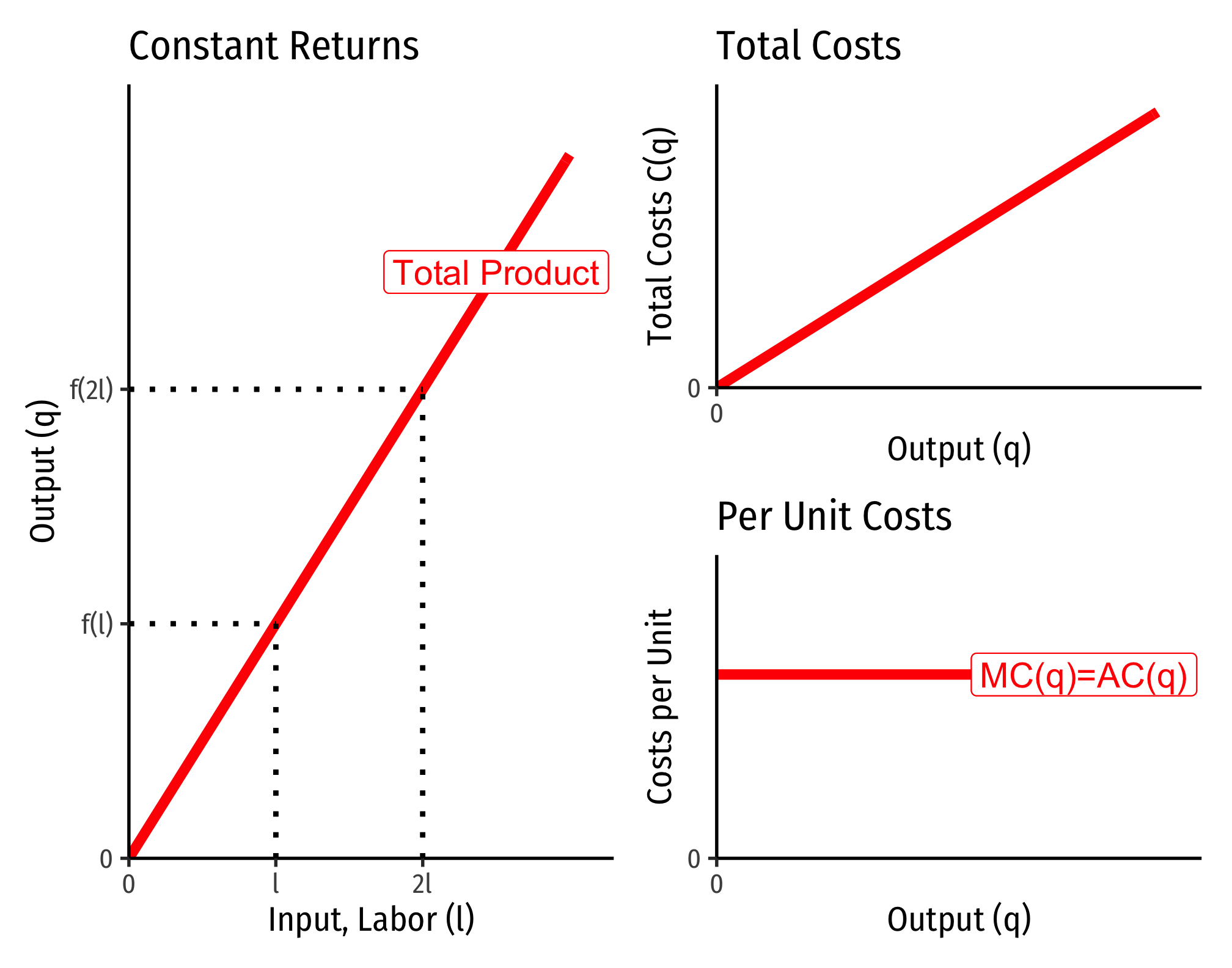
Constant Returns to Scale:

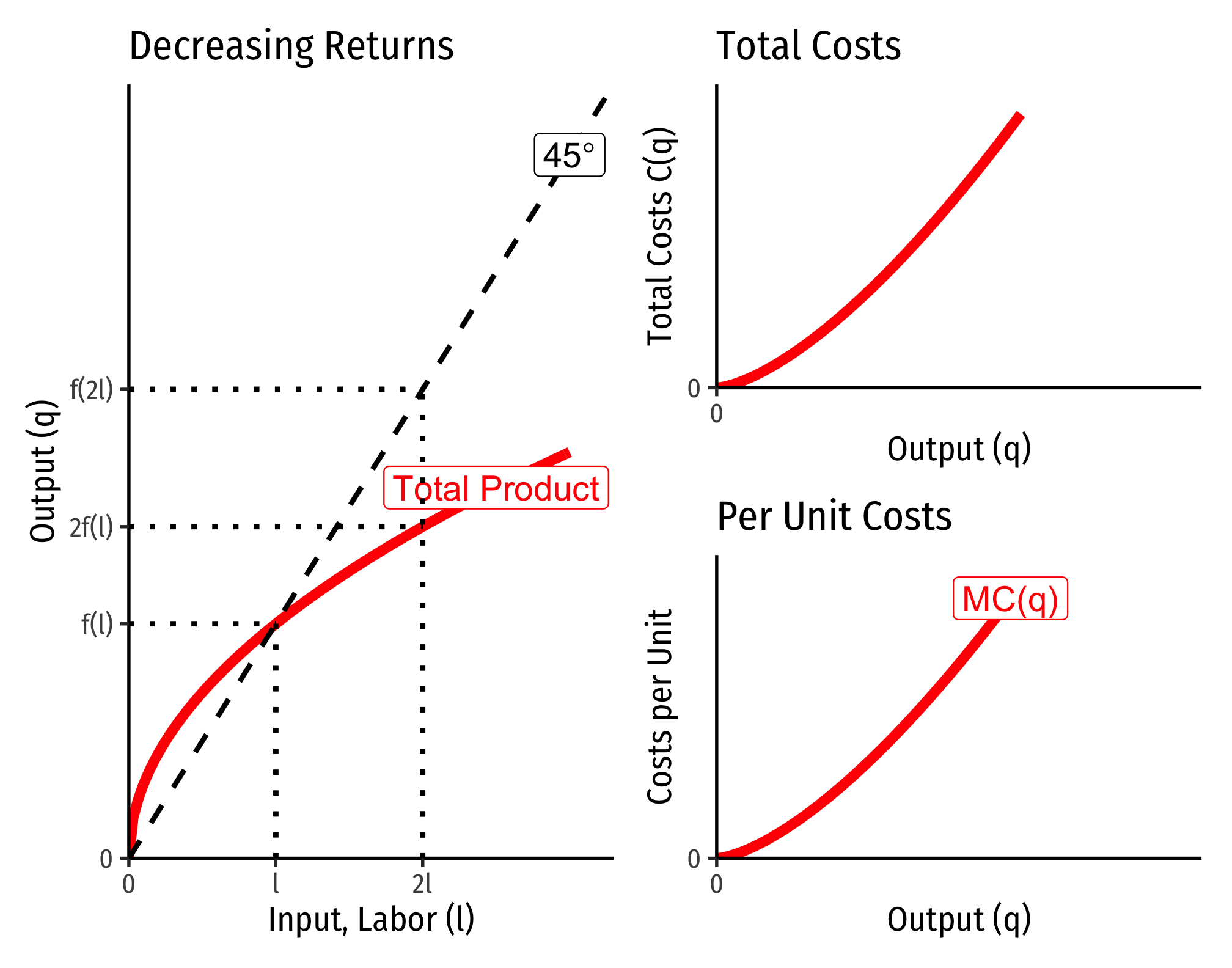
Decreasing Returns to Scale

Increasing Returns to Scale

Cobb-Douglas Cost Functions

The total cost function for Cobb-Douglas production functions of the form q=lαkβ

C(w,r,q)=[(αβ)βα+β+(αβ)−αα+β]wαα+βrβα+βq1α+β

If you take the first derivative of this (to get marginal cost), it is:

∂C(w,r,q)∂q=MC(q)=1α+β(wαα+βrβα+β)q(1α+β)−1

How does marginal cost change with increased output? Take the second derivative:

∂2C(w,r,q)∂q2=1α+β(1α+β−1)(wαα+βrβα+β)q(1α+β)−2

Three possible cases:

1. If 1α+β>1, this is positive ⟹ decreasing returns to scale

• Production function exponents α+β<1

2. If 1α+β<1, this is negative ⟹ increasing returns to scale

• Production function exponents α+β>1

3. If 1α+β=1, this is constant ⟹ constant returns to scale

• Production function exponentsα+β=1

Example (Constant Returns)

Let q=l0.5k0.5.

C(w,r,q)=[(0.50.5)0.50.5+0.5+(0.50.5)−0.50.5+0.5]w0.50.5+0.5r0.50.5+0.5q10.5+0.5C(w,r,q)=[10.5+1−0.5]w0.5r0.5q0.5C(w,r,q)=w0.5r0.5q1

Consider input prices of w=$9 and r=$25:

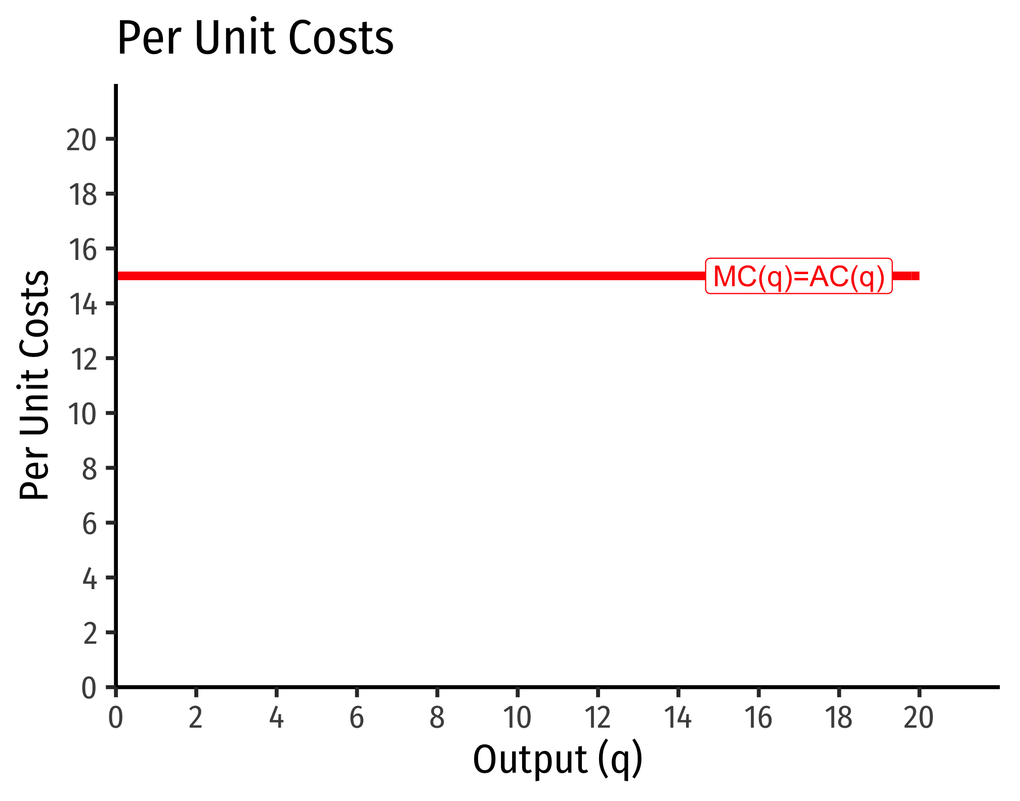
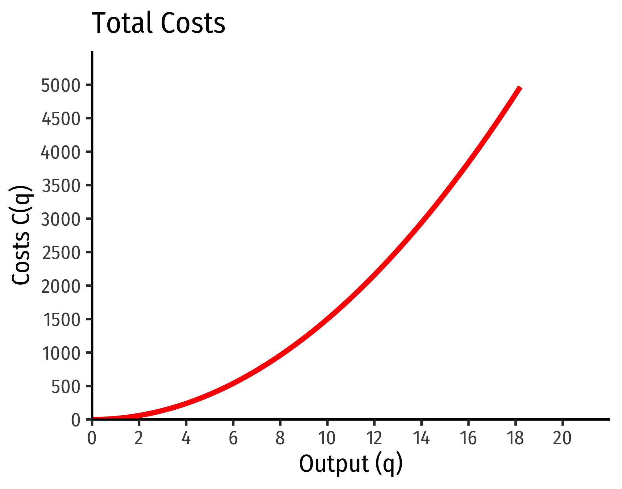
C(w=10,r=20,q)=90.5250.5q=3∗5∗q=15q

That is, total costs (at those given input prices, and technology) is equal to 15 times the output level, q:

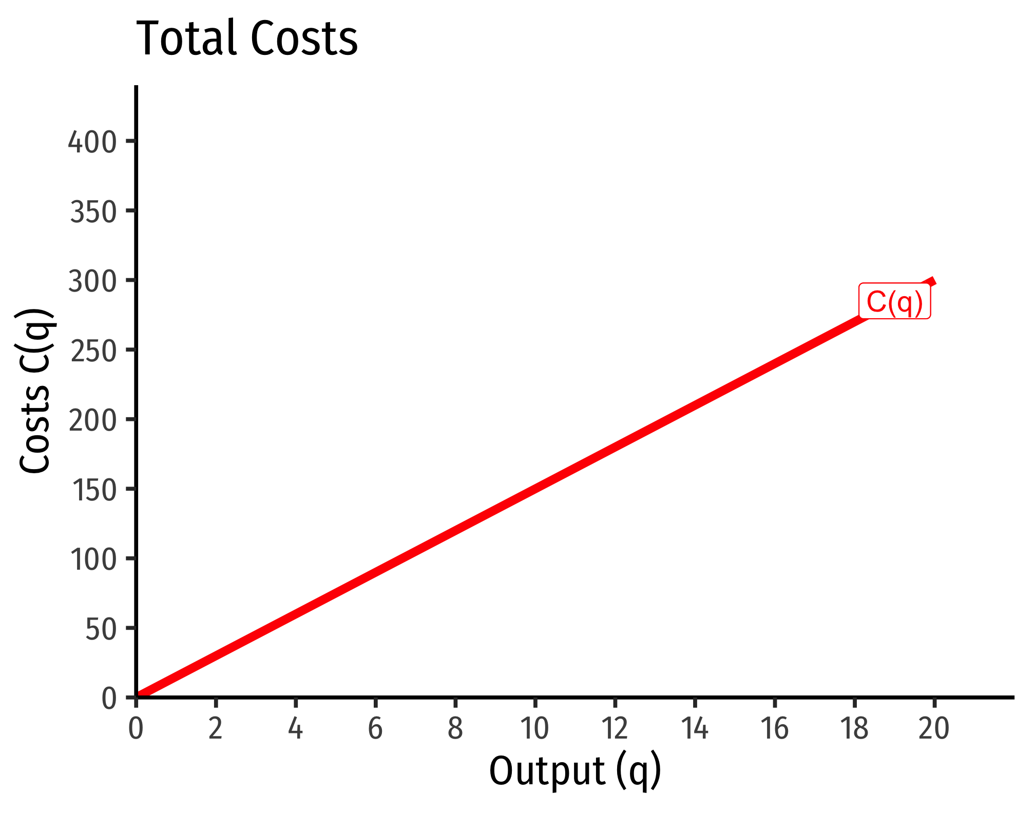
Marginal costs would be

MC(q)=∂C(q)∂q=15

Average costs would be

MC(q)=C(q)q=15qq=15

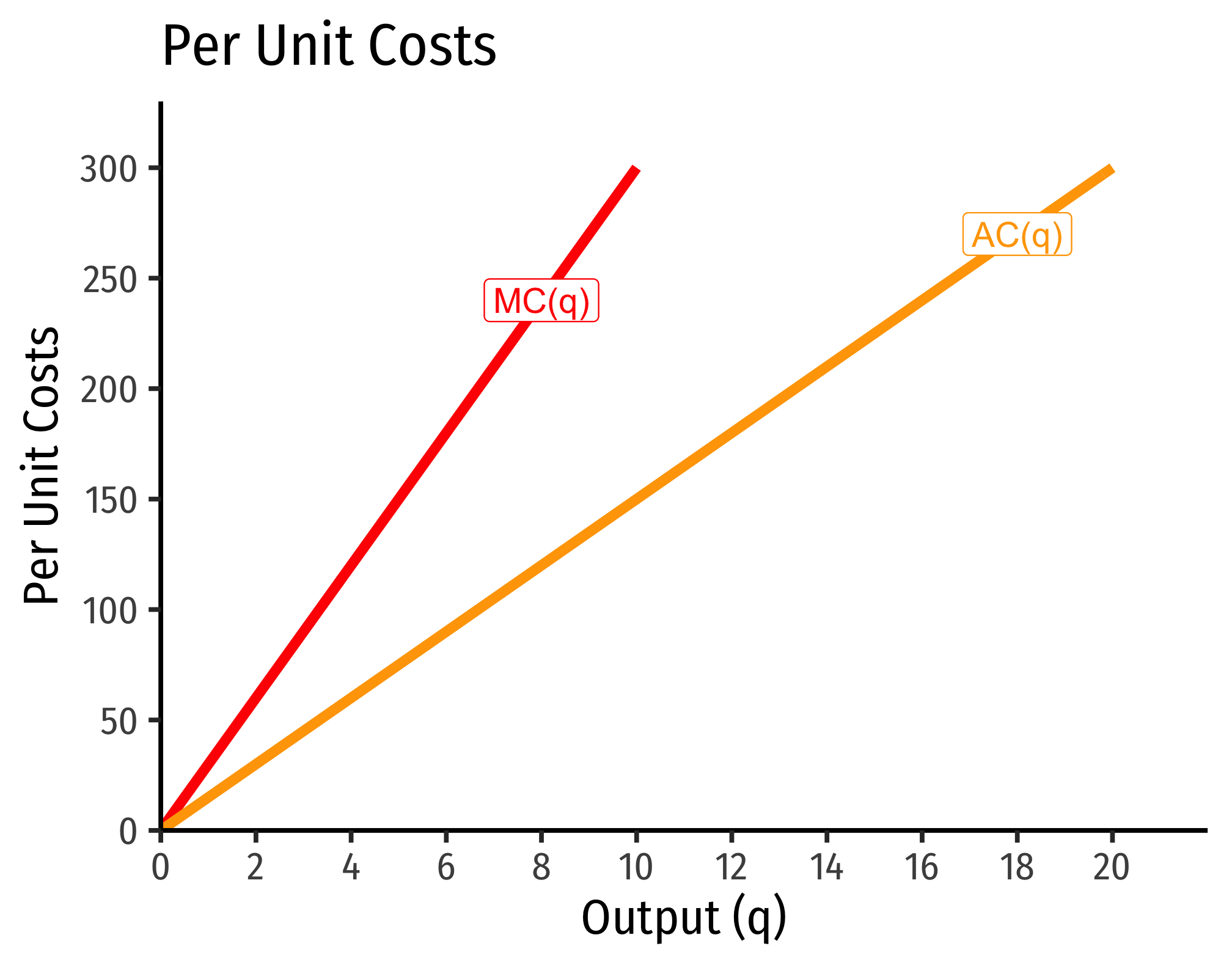
Example (Decreasing Returns)

Let q=l0.25k0.25.

C(w,r,q)=[(0.250.25)0.250.25+0.25+(0.250.25)−0.250.25+0.25]w0.250.25+0.25r0.250.25+0.25q10.25+0.25C(w,r,q)=[10.5+1−0.5]w0.5r0.5q2C(w,r,q)=w0.5r0.5q2

If w=9, r=25:

C(w=10,r=20,q)=90.5250.5q2=3∗5∗q2=15q2

Marginal costs would be

MC(q)=∂C(q)∂q=30q

Average costs would be

AC(q)=C(q)q=15q2q=15q