4.1 — Modeling Firms With Market Power — Class Notes
Contents
Monday, November 2, 2020
Overview
Today we begin our look at “imperfect competition,” where firms have market power, meaning they can charge p>MC and search for the profit-maximizing quantity and price. Today is merely about how do change the model to understand how a firm with market power behaves. To assist us, we begin with an extreme case of a single seller, i.e. a monopoly. For now we only assume that there is a single firm, and see how it behaves differently than if it were in a competitive market. Next class we will begin to explore what could cause a market to have only a single seller, and what are some of the social consequences of market power.
Readings
See today’s suggested readings.
Slides
Practice Problems
Today you will be working on practice problems. Answers will be posted there later.
Assignments: Problem Set 5 (Due Sun Nov 8)
Homework 5 (on 3.1-3.5) is due by PDF upload to Blackboard by 11:59 PM Sunday November 8. This is likely your final graded homeworkIn the past, I have always released a HW 6 on Imperfect Competition just for practice for the Final Exam.
Appendix
Monopolists Only Produce Where Demand is Elastic: Proof
Let’s first show the relationship between MR(q) and price elasticity of demand, ϵD.
MR(q)=p+(ΔpΔq)qDefinition of MR(q)MR(q)p=pp+(ΔpΔq)qpDividing both sides by pMR(q)p=1+(ΔpΔq×qp)⏟1ϵSimplifyingMR(q)p=1+1ϵDRecognize price elasticity ϵD=ΔqΔp×pqMR(q)=p(1+1ϵD)Multiplying both sides by p
Remember, we’ve simplified ϵD=1slope×pq, where 1slope=ΔqΔp because on a demand curve, slope=ΔpΔq.
Now that we have this alternate expression for MR(q), lets assume MC(q)≥0 and set them equal to one another to maximize profits:
MR(q)=MC(q)p(1+1ϵD)=MC(q)p(1−1|ϵD|)=MC(q)
I rearrange the last line only to remind us that ϵD is always negative!
Now note the following:
- If |ϵD|<1, then MR(q) is negative. Since MC(q) is assumed to be positive, it cannot equal a negative MR(q), hence this is not profit-maximizing.
- If |ϵD|=1, then MR(q) is 0. Only if MC(q) is also 0 is this profit-maximizing.
- If |ϵD|>1, then MR(q) is positive. It can equal a positive MC(q) to be profit-maximizing.
Hence, a monopolist will never produce in the inelastic region of the demand curve (where MR(q)<0), and will only produce at the unit elastic part of the demand curve (where MR(q)=0) if MC(q)=0. Thus, it generally produces in the elastic region where MR(q)>0.
See the graphs on slide 31.
Derivation of the Lerner Index
Marginal revenue is strongly related to the price elasticity of demand, which is ED=ΔqΔp×pqI sometimes simplify it as ED=1slope×pq, where “slope” is the slope of the inverse demand curve (graph), since the slope is ΔpΔq=riserun.
We derived marginal revenue (in the slides) as:
MR(q)=p+ΔpΔqq
Firms will always maximize profits where:
MR(q)=MC(q)Profit-max outputp+(ΔpΔq)q=MC(q)Definition of MR(q)p+(ΔpΔq)q×pp=MC(q)Multiplying the left by pp (i.e. 1)p+(ΔpΔq×qp)⏟1ϵ×p=MC(q)Rearranging the leftp+1ϵ×p=MC(q)Recognize price elasticity ϵ=ΔqΔp×pqp=MC(q)−1ϵpSubtract 1ϵp from both sidesp−MC(q)=−1ϵpSubtract MC(q) from both sidesp−MC(q)p=−1ϵDivide both sides by p
The left side gives us the fraction of price that is markup (p−MC(q)p), and the right side shows this is inversely related to price elasticity of demand.
Differences Between Firms With Market Power and Competitive Firms
Firms respond to changes in the marketplace differently depending on whether they have market power or not (are price-takers in perfect competition). Let’s examine three cases to see how each type of firm optimally responds to changes in key parameters: a change in costs, a shift in demand, and a change in price elasticity of demand.
First, compare the two types of firms — a price-taker in perfect competition on the left, and a firm with market power on the right.
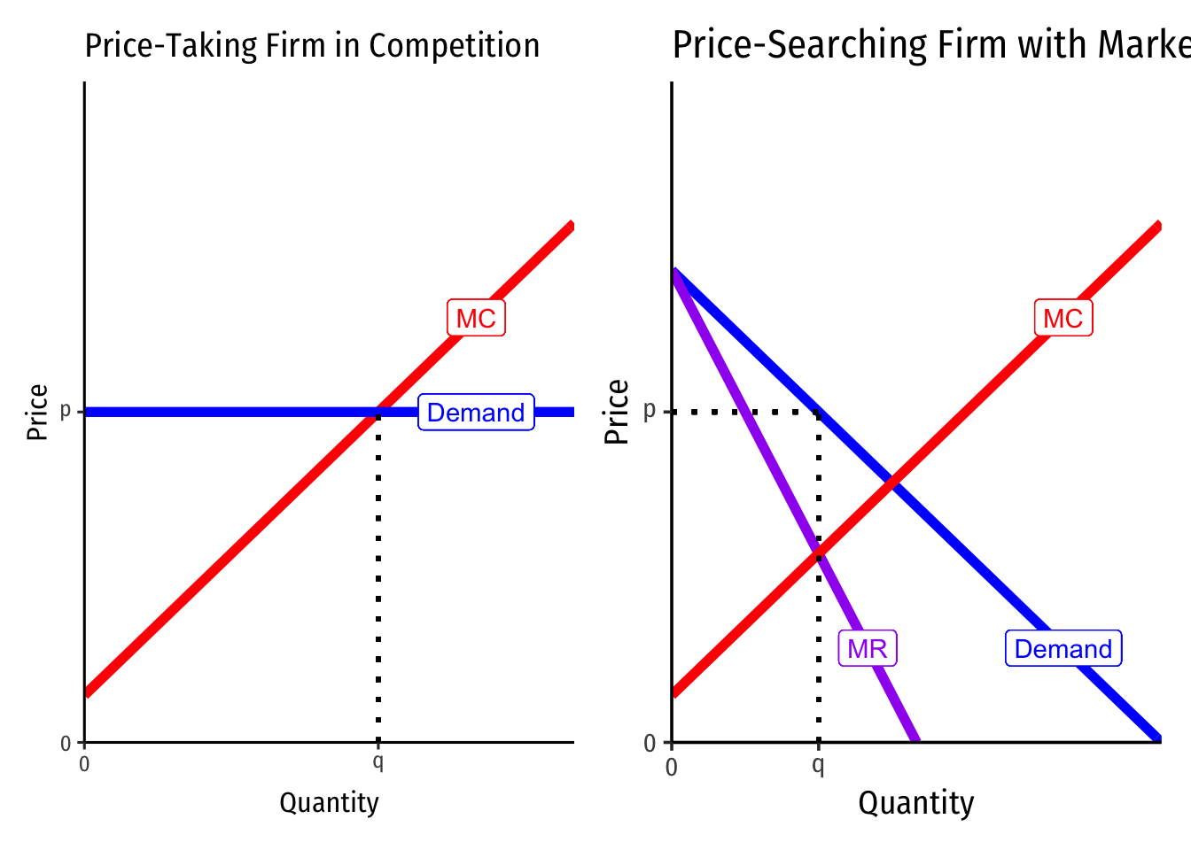
Again, notice the competitive firm has a perfectly elastic demand at the market-determined priceThis is not shown, but imagine a full market supply and demand graph that intersect at the market clearing equilibrium price, which this representative firm takes as given.
and sets p=MC (since it sets MR=MC and MR=p) to produce the optimal profit-maximizing quantity.
And also notice the firm with market power faces the full downward-sloping market demand curve for its product, and this implies a separate marginal revenue curve (with twice the slope of the demand curve). This firm first sets MR=MC to determine the optimal profit-maximizing quantity, and then raises price up to the maximum consumers are willing to pay (their Demand at that quantity).
A Change in Marginal Cost
Suppose both types of firms see an increase in their costs. Perhaps this is the result of a specific excise (per-unit) tax placed on the firm’s sales, raising the marginal cost by a fixed amount.
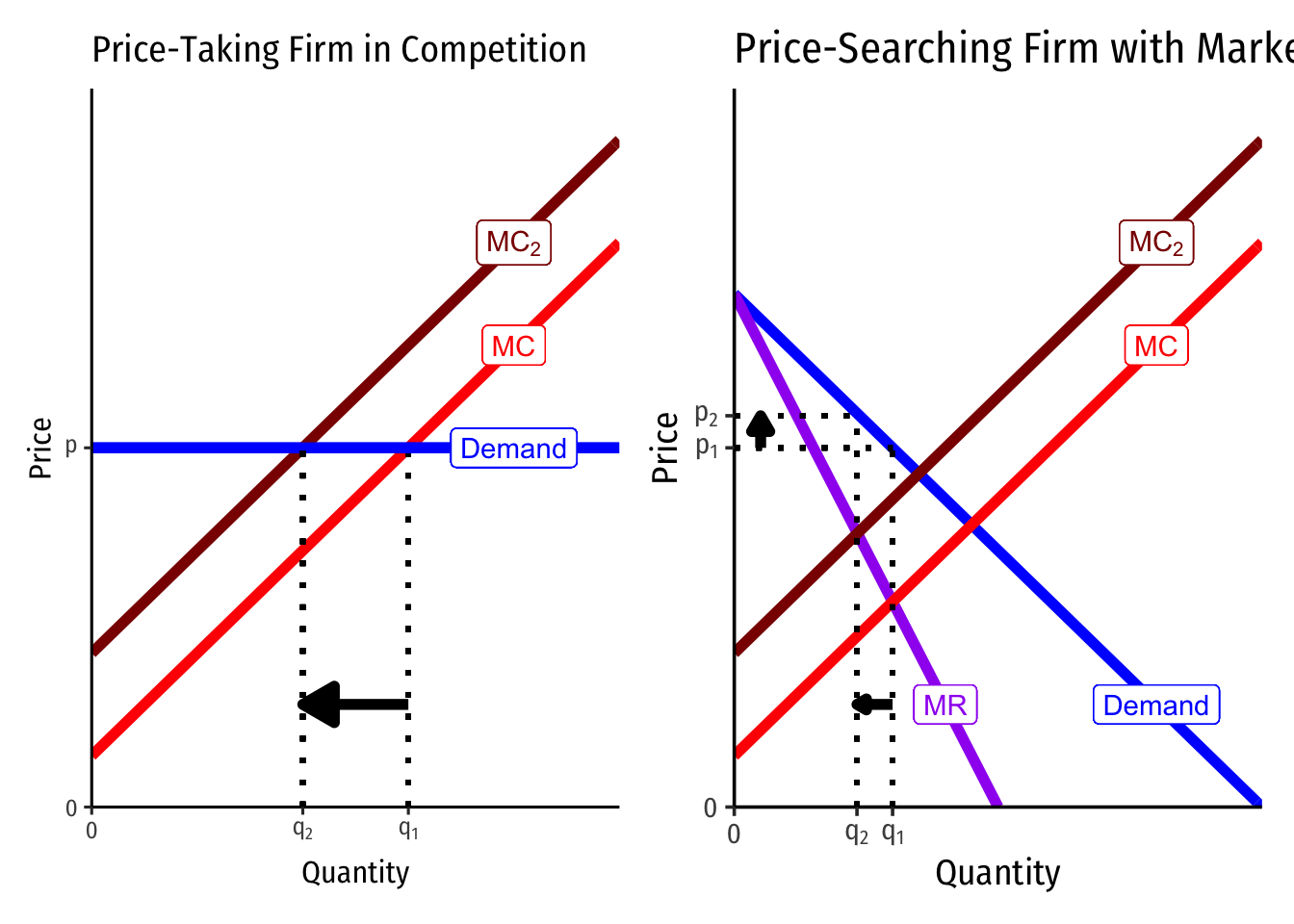
Notice that both firms see their marginal costs shift upwards by the same amount.
Because there is no slope to the competitive firm’s demand curve, the price remains unchanged, but the optimal quantity decreases.
Since there is a slope to the firm with market power, the price will change in addition to the quantity. Always setting (the new) MC=MR, the firm produces less output, and raises the price to the demand curve. At the smaller quantity, the willingness to pay is much higher.
Alternatively, we could imagine a fall in costs, by considering a change from MC2 to MC for each firm (and see how the opposite happens).
Thus, a key difference here is that a change in costs will only change quantity produced for the competitive firm, but will change both quantity and price for a firm with market power.
We are also ignoring average costs (not shown), which would affect profit. But this highlights that only changes in marginal cost affect the quantity of output produced.
Change in Demand
Suppose instead there is a change in market demand for the product.
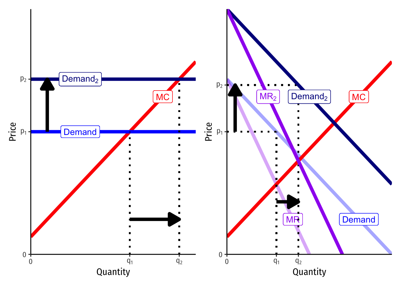
The competitive firm faces a higher demand at a (now higher) market-determined priceAgain, not not shown, but imagine the full market demand curve shifts to the right on the market supply and demand graph, intersecting at a higher market clearing equilibrium price, which this representative firm takes as given.
and sets p=MC (since it sets MR=MC and MR=p) to produce the optimal profit-maximizing quantity. Since the market price is higher, the firm produces a higher output at the higher price.
The firm with market power also sees an equivalent shift of market demand, and note that this also shifts the marginal revenue curve (always starting at the same point as market demand, with twice the slope). With an upward-sloping marginal cost curve and a downward-sloping marginal revenue curve, MR=MC will occur at a larger quantity than before (but notice a smaller increase than the competitive firm, where the demand & marginal revenue curves are horizontal), and again at a higher price.
Thus, both firms will see an increase in price and quantity from an increase in demand, but the firm with market power does not increase output as much as the competitive firm. Remember, a firm with market power generally wants to restrict output to raise its price compared to what a competitive market would do.
We can see the same thing in reverse for a decrease in market demand (move from Demand2 to Demand).
A Change in Price Elasticity of Market Demand
Finally, suppose the demand changes elasticity, but does not change the market price.This latter assumption is important in antitrust and economic regulation, for trying to decipher the difference between a competitive market and a cartel based on their prices.
Things like new competitors entering and creating more substitutes, would make demand more elastic. Both the less elastic (original) demand curve and the new, more elastic DemandE curve pass through the same optimal point.
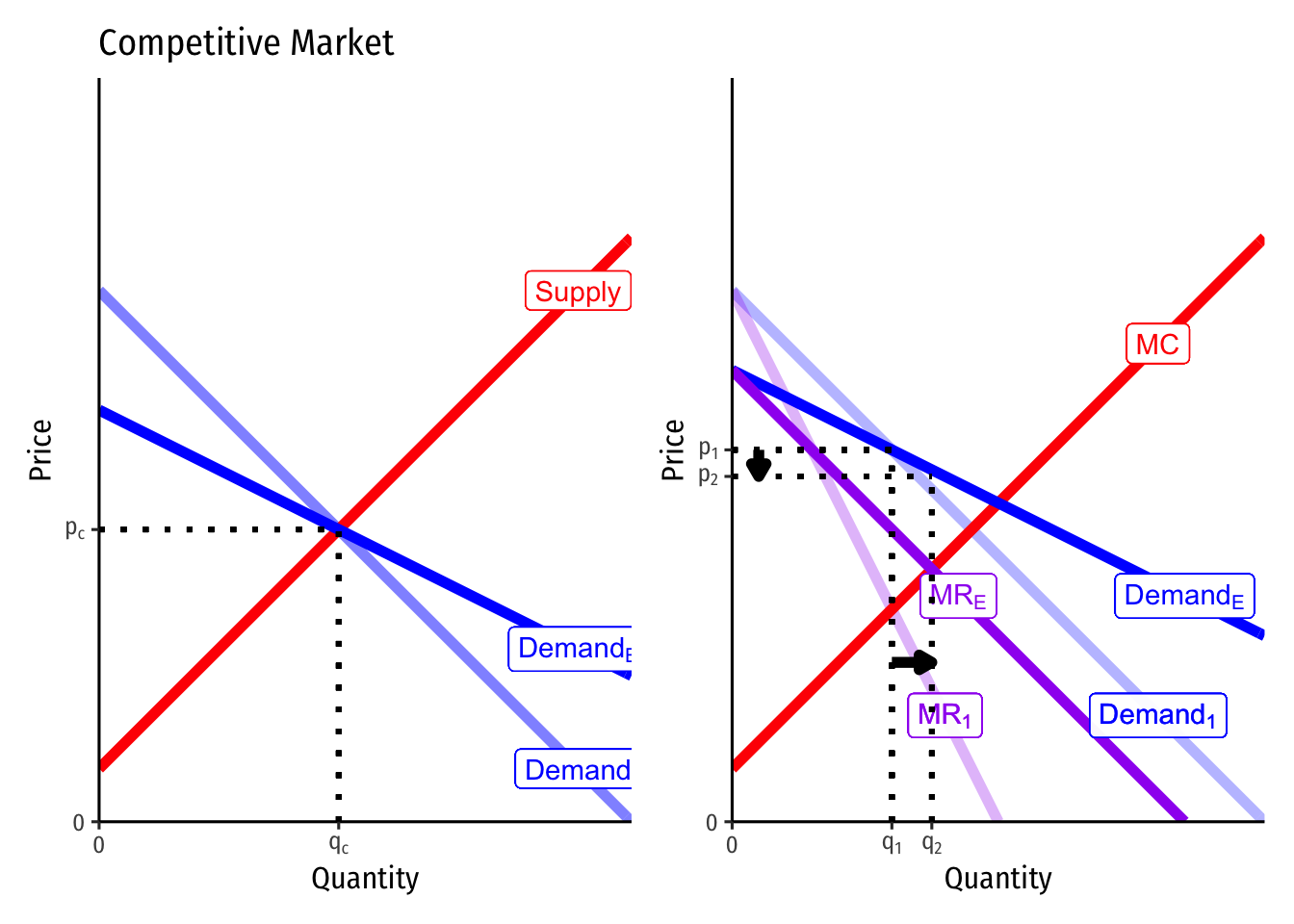
The left graph is now the market for the entire industry that is competitive, rather than for a representative firm in that market. Note the demands change elasticity, but do not affect the market-clearing equilibrium price or quantity. Hence, nothing will change in terms of price or output for the firms in this industry.
The right graph shows the change for a firm with market power. The more elastic demand curve DemandE rotates through the original optimum price and quantity (q1,q1). Since there is a new (flatter) demand curve, there is also a new (flatter) marginal revenue curve MRE. The firm sets this new MRE=MC to find that it should increase its quantity to q2 and lower its price to p2. Thus, as demand becomes more elastic, the firm produces more and lowers the price. The opposite would happen if demand became less elastic.