2.5 — Short Run Profit Maximization — Class Notes
Contents
Wednesday, September 30, 2020
Overview
Today we finish up costs from last lecture, and briefly discuss revenues before we put them together next class to solve the firm’s profit maximization problem. We focus on the short run, where the firm incurs fixed costs and must stay in the market regardless. We derive the firm’s (inverse) supply curve.
Next class will be about the long run, and finish up unit 2.
I have your Exam 1 graded and will discuss them at the end of class today. See assignments below for more information.
Slides
Practice Problems
Today we will be working on practice problems. Answers will be posted on that page.
Assignments
Homework 3 anawers are posted on that page.
Homework 4 will be posted shortly, and will be due by PDF upload on Blackboard by 11:59PM Sunday October 11.
Exam 1 corrections are due to me by an emailed PDF by 11:59 PM Sunday October 11. You may redo any question you did not get full points on (do not do questions you did not lose points on), including bonuses. Write the correct answer and explain why it’s the right answer (i.e. show your work, don’t just write “It’s inelastic” when you wrote “elastic” on the exam.) I want you to demonstrate you are internalizing the answers and learning, not just comparing with your friends to get the correct answer. You can talk to each othjer now, and are welcome to come to my (and the TAs’) office hours to go over the exam together.
We will wrap up Unit 2 next Monday. Wewe will hold a review session on Wednesday (October 7), and have Exam 2 the following week (week of October 12). This time, we will not have class on Monday October 12, to help facilitate you taking the next exam.
Appendix
Common Cost Assumptions
Economists often make simple assumptions about costs to illustrate key concepts without marring the analysis with unnecessary complexity. This also makes graphs quite easy to point to and calculate key ares, such as profits or deadweight losses.
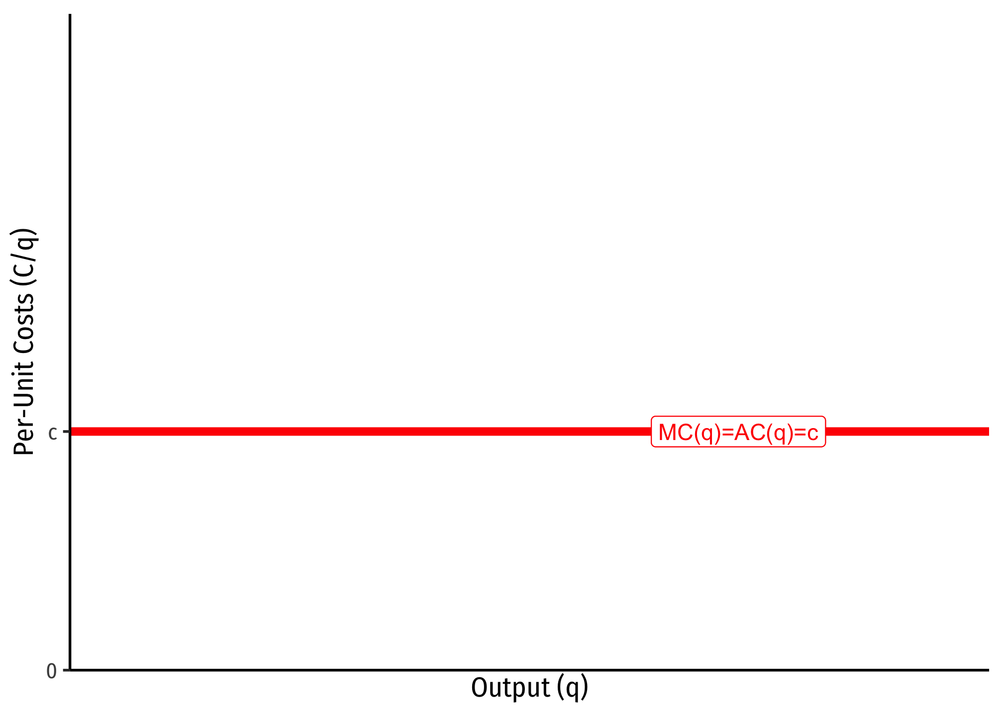
One common set of cost assumptions is the following:
- A firm has no fixed costs
- A firm has constant marginal costs, MC(q)=c where c≥0
If this is the case, then we can show that average costs will be equal to marginal costs, i.e. MC=AC=AVC=c.
Since marginal cost is the first derivative of the total cost function, integrating a marginal cost function MC=c leaves with with a total cost function of C(q)=cq.Since we assumed there are no fixed costs, then there is no arbitrary constant from integration.
If this is the case, then we can find the average cost:
C(q)=cqAC(q)=C(q)q=cqqAC(q)=c
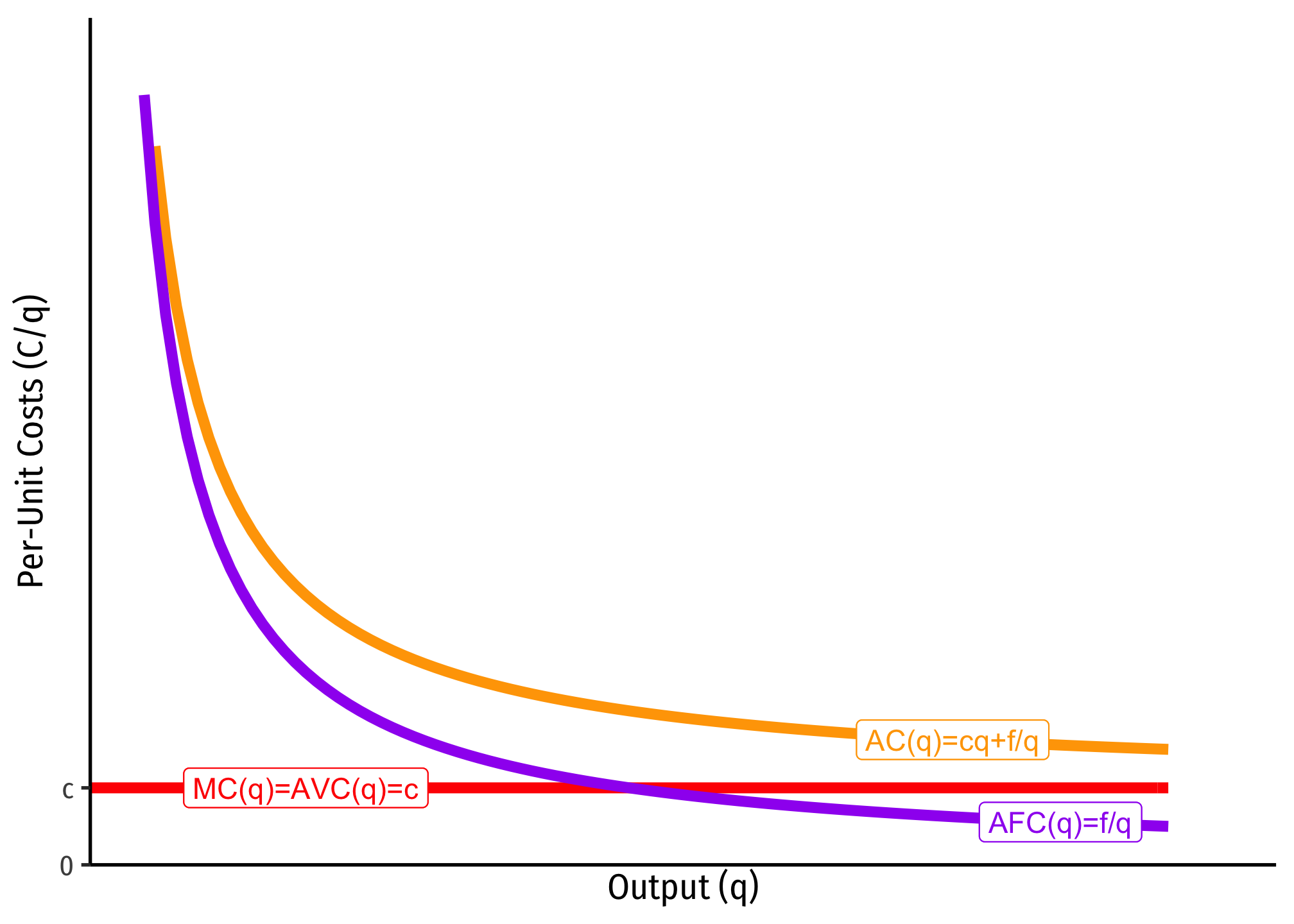
Another common set of cost assumptions is the following:
- A firm has fixed costs, f
- A firm has constant marginal costs, MC(q)=c where c≥0
If this is the case, then we can show that average costs are strictly decreasing over all output q≥0.
Again, we can integrate marginal cost to the total cost function (but here we need the arbitrary constant from integration, which we shall label f, for fixed costs): C(q)=cq+f. We can then find the average cost:
C(q)=cq+fAC(q)=C(q)q=cq+fqAC(q)=c+fq
Since f>0, as q→∞, AC(q)→c, that is, average cost is getting asymptotically close to marginal cost, c, but will never intersect it. Note, I also included AFC, which again is always decreasing, and asymptotically approaching 0.
The importance of this type of cost structure is that it creates economies of scale, and represents a lot of industries that tend towards natural monopoly.